一致性预测模型¶

以下是 Darts 中一致性预测模型的演示。

总结：

Darts 中的一致性预测构造有效的预测区间，无需分布假设。
由于其简单性和效率，我们使用分割一致性预测 (SCP)。
您可以将一致性预测应用于任何预训练的全局预测模型。
为了改善您的体验，我们的一致性模型会自动从输入序列中提取生成区间所需的校准数据。
我们提供有用的特性来配置提取过程，使您的一致性模型更具适应性和效率 (cal_length, cal_stride)。
一致性预测支持所有用例（单变量和多变量，单系列和多系列，单步和多步预测，提供直接分位数预测值或采样预测）。
我们将通过四个使用真实世界数据的示例来演示如何使用和评估一致性预测。

[1]:

# fix python path if working locally
from utils import fix_pythonpath_if_working_locally

fix_pythonpath_if_working_locally()

[2]:

%load_ext autoreload
%autoreload 2
%matplotlib inline
import matplotlib.pyplot as plt
import numpy as np
import pandas as pd

from darts import concatenate, metrics
from darts.datasets import ElectricityConsumptionZurichDataset
from darts.models import ConformalNaiveModel, ConformalQRModel, LinearRegressionModel

用于时间序列预测的一致性预测¶

一致性预测是一种构造预测区间的技术，它试图在有限样本中实现有效的覆盖率，无需分布假设。 (来源)

换句话说：如果我们想要一个在某个时间段内包含 80% 实际值的预测区间，那么一致性模型会尝试生成这样的区间，使 80% 的点实际落在其中。

有不同的技术来执行一致性预测。在 Darts 中，我们目前使用分割一致性预测 (SCP, Lei et al., 2018)（并进行了一些不错的调整），因为它简单高效。

分割一致性预测¶

SCP 为基础模型的预测添加具有指定置信水平的校准预测区间。它涉及将数据分割成训练（+可选验证）集和校准（+测试）集。模型在训练集上训练，校准集用于计算预测区间，以确保它们以期望的概率包含真实值。

优点¶

有效覆盖率：提供有效的预测区间，保证在有限样本中以指定置信水平包含真实值。
模型无关：可应用于任何预测模型
- 为点预测模型添加校准预测区间
- 或在概率预测模型的情况下校准预测区间
无分布假设：除了校准集上的误差是可交换的之外，没有关于数据的分布假设（例如，我们不需要假设数据是正态分布的，然后拟合一个带有 GaussianLikelihood 的模型）。
高效：分割一致性预测是高效的，因为它不需要重新训练模型。
可解释：由于其简单性，该方法具有可解释性。
有用的应用：它用于提供更可靠、信息更丰富的预测，以帮助多个行业的决策。请参阅这篇关于一致性预测的文章

缺点¶

需要校准集：一致性预测需要另一个数据/保留集，专门用于计算校准预测区间。这对于小数据集来说可能效率不高。
校准数据的可交换性 (a)：预测区间的准确性取决于校准数据的代表性（或者更确切地说，是在校准集上产生的预测误差）。如果预测误差存在分布偏移（例如，具有趋势的序列，但预测模型无法预测该趋势），则无法保证覆盖率。
保守性 (a)：可能会产生比必要更宽的区间，导致预测保守。

Darts 一致性模型有一些参数可以控制校准集的提取，以提高适应性（更多信息请参见此处）。

Darts 一致性模型¶

Darts 的一致性模型为任何预训练的全局预测模型的预测添加校准预测区间。无需训练一致性模型本身（例如，无需 fit()），您可以直接调用 predict() 或 historical_forecasts()。在内部，Darts 会自动从输入序列的历史数据中提取校准集，并使用它来生成校准预测区间（更多详情请参见此处）。

重要：传递给预测方法的 series 不应与用于训练预测模型的序列有任何重叠，否则将导致过于乐观的预测区间。

模型支持¶

Darts 中的所有一致性模型都支持

任何预训练的全局预测模型作为基础预测器（您可以在此处找到列表）
单变量和多变量预测（单列/多列）
单系列和多系列预测
单步和多步预测
生成单个或多个校准预测区间
这些分位数值的直接分位数值预测（区间边界）或采样预测
基于底层预测模型的任何协变量

直接区间预测或采样预测¶

一致性模型是概率性的，因此您可以通过两种方式进行预测（调用 predict(), historical_forecasts() 等时）

直接预测校准后的分位数区间边界（此处有示例）。
- predict(..., predict_likelihood_parameters=True)
通过从这些校准后的分位数区间中采样来生成随机预测（此处有示例）
- predict(..., num_samples=1000)

内部工作流程¶

注意：cal_length 和 cal_stride 将在下面进一步解释。

一般来说，模型产生一个校准预测/预测的工作流程如下（使用 predict()）

提取校准集：每个一致性预测的校准集都自动从输入序列相对于预测起始点的最新历史中提取。要考虑的校准示例数量（预测误差/不一致性分数）可以在模型创建时通过参数 cal_length 定义。请注意，当使用 cal_stride>1 时，需要更长的历史，因为校准示例是通过步长历史预测生成的。
在校准集上（使用预测模型）生成步长为 cal_stride 的历史预测。
计算这些历史预测上的误差/不一致性分数（特定于每个一致性模型）
从误差/不一致性分数中计算分位数值（使用我们在模型创建时通过参数 quantiles 设置的所需分位数）。
计算一致性预测：使用这些分位数值，为预测模型的预测添加校准区间（或调整现有区间）。

对于多步预测，以上过程对预测范围内的每一步单独应用。

计算 historical_forecasts(), backtest(), residuals() 等时，以上过程对每个预测都应用（预测模型的历史预测仅生成一次以提高效率）。

可用的一致性模型¶

截至本文撰写时（Darts 版本 0.32.0），我们有两个一致性模型

`ConformalNaiveModel`¶

在任何预训练的全局预测模型的中值预测周围添加校准区间。它支持两种对称模式

symmetric=True:
- 下限和上限区间以相同的幅度进行校准。
- 不一致性分数：使用绝对误差 ae() 在校准集上计算不一致性分数。
symmetric=False
- 下限和上限区间分别进行校准。
- 不一致性分数：使用误差 err() 在校准集上计算上限的不一致性分数，使用 -err() 计算下限的不一致性分数。

`ConformalQRModel` (一致化分位数回归模型)¶

校准预训练的概率全局预测模型的分位数预测。它支持两种对称模式

symmetric=True:
- 下限和上限分位数预测以相同的幅度进行校准。
- 不一致性分数：使用分位数回归不一致性分数 incs_qr(symmetric=True) 在校准集上计算。
symmetric=False
- 下限和上限分位数预测分别进行校准。
- 不一致性分数：使用分位数回归非对称不一致性分数 incs_qr(symmetric=False) 在校准集上计算上限和下限的不一致性分数。

Darts 特性，使您的一致性模型更具适应性¶

如分割一致性预测 - 缺点中所述，校准集对我们的一致性预测技术的有效性有很大影响。

我们实现了一些很酷的特性，使我们的校准集自动提取对您来说更强大。

我们所有的一致性模型在模型创建时都有以下两个参数

cal_length：在最近历史中使用的不一致性分数 (NCS) 的数量，用于每个一致性预测（和预测范围中的每一步）的校准。
- 如果为 None，则采用扩展窗口模式
- 如果 >=1，则使用移动固定长度窗口模式
- 优点
  - 使用 cal_length 可以使您的模型更快地对 NCS 的分布变化做出反应。
  - 使用 cal_length 可以降低执行校准的计算成本。
- 注意：使用足够大的值以获得足够的校准示例。
cal_stride：（默认=1）在校准集上计算历史预测和不一致性分数时应用的步长（连续两个预测之间的时间步数）。
- 如果您想按计划运行模型（例如，每 24 小时一次），并且只对在该计划下产生的 NCS 感兴趣，这将非常有用。
- 注意：cal_stride>1 需要更长的 series 历史记录（大约需要 cal_length * stride 个点）。

示例¶

我们将展示四个示例

如何执行一致性预测并根据量化的不确定性比较不同的模型。为简单起见，我们将使用单步预测范围 n=1。
如何执行多步一致性预测
如何按计划执行多步一致性预测
一致化分位数回归的示例。

输入数据集¶

对于这两个示例，我们使用来自瑞士苏黎世家庭的电力消费数据集。

数据集的频率是刻钟（15分钟间隔），但为了简单起见，我们将其重采样到小时频率。

为了简单起见，我们将不使用任何协变量，只关注作为我们想要预测的目标的电力消费。一致性模型的协变量支持和 API 与基础预测器相同。

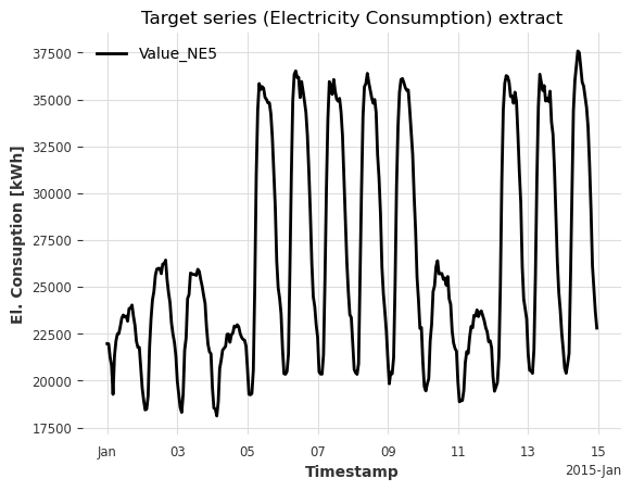
目标序列（我们想要预测的序列）：- Value_NE5：电网等级 5 的家庭电力消费（单位：千瓦时）。

[3]:

series = ElectricityConsumptionZurichDataset().load().astype(np.float32)

# extract target and resample to hourly frequency
series = series["Value_NE5"].resample(freq="h")

# plot 2 weeks of hourly consumption
ax = series[: 2 * 7 * 24].plot()
ax.set_ylabel("El. Consuption [kWh]")
ax.set_title("Target series (Electricity Consumption) extract");

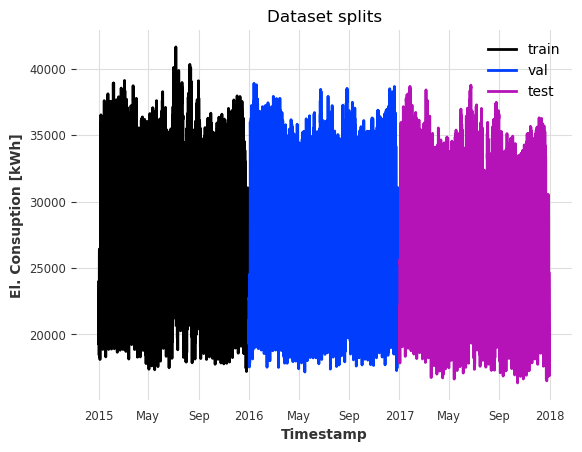
../_images/examples_23-Conformal-Prediction-examples_6_0.png

提取训练集、校准集和测试集。注意，cal 不与训练集 train 重叠。

[4]:

train_start = pd.Timestamp("2015-01-01")
cal_start = pd.Timestamp("2016-01-01")
test_start = pd.Timestamp("2017-01-01")
test_end = pd.Timestamp("2018-01-01")

train = series[train_start : cal_start - series.freq]
cal = series[cal_start : test_start - series.freq]
test = series[test_start:test_end]

ax = train.plot(label="train")
cal.plot(label="val")
test.plot(label="test")

ax.set_ylabel("El. Consuption [kWh]")
ax.set_title("Dataset splits");

../_images/examples_23-Conformal-Prediction-examples_8_0.png

示例 1：比较单步预测的不同模型¶

让我们看看如何在 Darts 中使用一致性预测。我们将展示如何

使用一致性预测（预测和历史预测）
评估预测区间（简单预测和回测）。
使用一致性预测比较两个不同的基础预测模型。

为了演示该过程，我们首先只关注一个基础预测模型。

训练基础预测器¶

让我们使用 LinearRegressionModel 作为我们的基础预测模型。我们将其配置为使用最后两个小时作为回溯窗口来预测下一小时（单步预测范围；多步预测将在示例 2 中介绍）。

在 train 集上训练它
预测 cal 集结束后的下一小时

[5]:

horizon = 1

# train the model
model = LinearRegressionModel(lags=2, output_chunk_length=horizon)
model.fit(train)

# forecast
pred = model.predict(n=horizon, series=cal)

# plot
ax = series[pred.start_time() - 7 * 24 * series.freq : pred.end_time()].plot(
    label="actual"
)
pred.plot(label="pred")
ax.set_title("First 1-step point prediction");

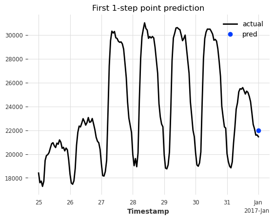
../_images/examples_23-Conformal-Prediction-examples_10_0.png

太棒了，我们有了单步预测。但是，如果我们不知道当时的实际目标值，我们就无法估计不确定性。

应用一致性预测¶

现在让我们应用一致性预测来量化不确定性。我们使用对称（默认）朴素模型，包括我们想要预测的分位数水平。此外

我们不需要训练/拟合一致性模型
我们应该向 predict() 提供一个与用于训练模型的序列没有重叠的 series。在我们的例子中，cal 与 train 没有重叠。
API 与 Darts 的预测模型相同。

让我们配置一致性模型：- 添加一个 90% 的分位数区间（分位数 0.05 - 0.95）（quantiles）。- 只考虑最近 4 周的不一致性分数来校准预测区间（cal_length）。

注意：您可以添加任意数量的区间，例如 [0.10, 0.20, 0.50, 0.80, 0.90] 将添加 80% (0.10 - 0.90) 和 60% (0.20 - 0.80) 的区间

[6]:

quantiles = [0.05, 0.50, 0.95]
four_weeks = 4 * 7 * 24
pred_kwargs = {"predict_likelihood_parameters": True, "verbose": True}

# create conformal model
cp_model = ConformalNaiveModel(model=model, quantiles=quantiles, cal_length=four_weeks)

# conformal forecast
pred = cp_model.predict(n=horizon, series=cal, **pred_kwargs)

# plot
ax = series[pred.start_time() - 7 * 24 * series.freq : pred.end_time()].plot(
    label="actual"
)
pred.plot(label="cp")
ax.set_title("First 1-step conformal prediction");

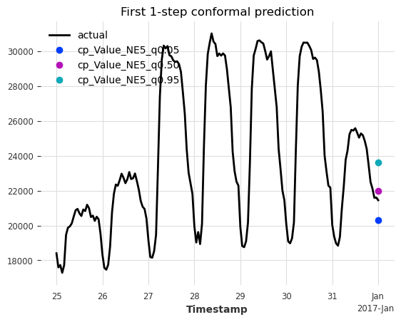
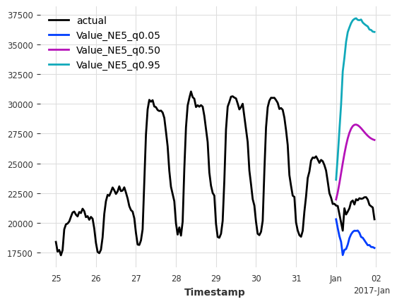
../_images/examples_23-Conformal-Prediction-examples_13_2.png

太棒了，我们可以看到在基础模型的预测（紫色）周围添加了预测区间（青绿色，深蓝色）。很明显，预测区间包含了实际值。让我们看看如何评估这个预测。

评估一致性预测¶

Darts 为预测区间提供了专门的指标。您可以在我们的指标页面的“分位数区间指标”下找到它们。您可以将它们用作独立指标或用于回测。

(m)ic：（平均）区间覆盖率
(m)iw：（平均）区间宽度
(m)iws：（平均）区间温克勒得分
(m)incs_qr：（平均）分位数回归不一致性分数

注意：对于 backtest()，请使用 (m)ean 指标，例如 mic()；对于 residuals()，请使用按时间步计算的指标，例如 ic()。

让我们检查一下区间覆盖率（每个区间内包含实际值的比例）和区间宽度

[7]:

q_interval = cp_model.q_interval  # [(0.05, 0.95)]
q_range = cp_model.interval_range  # [0.9]


def compute_metrics(pred_):
    mic = metrics.mic(series, pred_, q_interval=q_interval)
    miw = metrics.miw(series, pred_, q_interval=q_interval)
    return pd.DataFrame({"Interval": q_range, "Coverage": mic, "Width": miw}).round(2)


compute_metrics(pred)

[7]:

	区间	覆盖率	宽度
0	0.9	1.0	3321.12

好的，我们看到区间宽度为 3.3 MWh，覆盖率为 100%。我们预期覆盖率为 90%（在有限样本上）。但到目前为止，我们只看了一个示例。它在整个测试集上的表现如何？

[8]:

# concatenate cal and test set to be able to start forecasting at the `test` start time
cal_test = concatenate([cal, test], axis=0)

hfcs = cp_model.historical_forecasts(
    series=cal_test,
    forecast_horizon=horizon,
    start=test.start_time(),
    last_points_only=True,  # returns a single TimeSeries
    **pred_kwargs,
)

[9]:

def plot_historical_forecasts(hfcs_):
    fig, (ax1, ax2) = plt.subplots(ncols=2, figsize=(16, 4.3))
    test[: 2 * 7 * 24].plot(ax=ax1)
    hfcs_[: 2 * 7 * 24].plot(ax=ax1)
    ax1.set_title("Predictions on the first two weeks")
    ax1.legend(loc="lower center", bbox_to_anchor=(0.5, -0.25), ncol=4, fontsize=9)

    test.plot(ax=ax2)
    hfcs_.plot(ax=ax2, lw=0.2)
    ax2.set_title("Predictions on the entire test set")
    ax2.legend(loc="lower center", bbox_to_anchor=(0.5, -0.25), ncol=4, fontsize=9)


plot_historical_forecasts(hfcs)

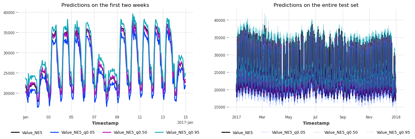
../_images/examples_23-Conformal-Prediction-examples_19_0.png

太棒了，我们刚刚在不到 1 秒的时间内完成了一年的一致性预测模拟！这些区间似乎也校准得很好。让我们通过计算所有历史预测（回测）的指标来找出答案。

[10]:

bt = cp_model.backtest(
    cal_test,
    historical_forecasts=hfcs,
    last_points_only=True,
    metric=[metrics.mic, metrics.miw],
    metric_kwargs={"q_interval": q_interval},
)
bt = pd.DataFrame({"Interval": q_range, "Coverage": bt[0], "Width": bt[1]})
bt

[10]:

	区间	覆盖率	宽度
0	0.9	0.901609	2908.944092

太棒了！我们的区间确实覆盖了所有实际值的 90%。平均宽度/不确定性范围略低于 3MWh。

看看覆盖率和宽度随时间的变化也会很有趣。

覆盖率指标 ic() 为每个时间步提供一个二进制值（区间是否包含实际值）。要获得某个时间段内的覆盖率比例，我们计算以 4 周为窗口的移动平均值。

[11]:

def compute_moving_average_metrics(hfcs_, metric=metrics.ic):
    """Computes the moving 4-week average of a specific time-dependent metric."""
    # compute metric on each time step
    residuals = cp_model.residuals(
        cal_test,
        historical_forecasts=hfcs_,
        last_points_only=True,
        metric=metric,
        metric_kwargs={"q_interval": q_interval},
    )

    # let's apply a moving average to the residuals with a winodow of 4 weeks
    windowed_residuals = residuals.window_transform(
        transforms={"function": "mean", "mode": "rolling", "window": four_weeks}
    )
    return windowed_residuals

[12]:

covs = compute_moving_average_metrics(hfcs, metrics.ic)
widths = compute_moving_average_metrics(hfcs, metrics.iw)

fig, (ax1, ax2) = plt.subplots(ncols=2, figsize=(12, 4.3))
covs.plot(ax=ax1, label="coverages")
ax1.set_ylabel("Ratio covered [-]")
ax1.set_title("Moving 4-week average of Interval Coverages")

widths.plot(ax=ax2, label="widths")
ax2.set_ylabel("Width [kWh]")
ax2.set_title("Moving 4-week average of Interval Widths");

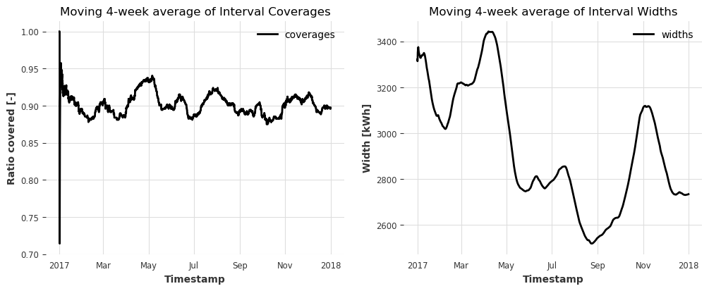
../_images/examples_23-Conformal-Prediction-examples_24_0.png

在这里，覆盖率在整个一年中也保持在 90% 左右，这表明一致性模型是有效的。

区间宽度范围从 2.5 到 3.5 MWh。宽度对模型性能变化的适应性/响应性主要由 cal_length 的值控制。

与另一个模型的比较¶

好的，现在让我们将第一个模型的不确定性与更强大的回归模型进行比较。

使用最近一周（7*24 小时）的消费作为回溯窗口
同时使用一天中小时和一周中天数的循环编码作为未来协变量

过程与第一个模型完全相同，所以我们不再赘述。

[13]:

add_encoders = {"cyclic": {"future": ["hour", "dayofweek"]}}
input_length = 7 * 24
model2 = LinearRegressionModel(
    lags=input_length,
    lags_future_covariates=(input_length, 1),
    output_chunk_length=1,
    add_encoders=add_encoders,
)
model2.fit(train)

cp_model2 = ConformalNaiveModel(
    model=model2, quantiles=quantiles, cal_length=four_weeks
)
hfcs2 = cp_model2.historical_forecasts(
    series=cal_test,
    forecast_horizon=horizon,
    start=test.start_time(),
    last_points_only=True,
    stride=horizon,
    **pred_kwargs,
)
plot_historical_forecasts(hfcs2)

bt2 = cp_model.backtest(
    cal_test,
    historical_forecasts=hfcs2,
    last_points_only=True,
    metric=[metrics.mic, metrics.miw],
    metric_kwargs={"q_interval": q_interval},
)
bt2 = pd.DataFrame({"Interval": q_range, "Coverage": bt2[0], "Width": bt2[1]})
bt2

[13]:

	区间	覆盖率	宽度
0	0.9	0.898413	1662.243896

../_images/examples_23-Conformal-Prediction-examples_27_3.png

太棒了！我们再次达到了 90% 的覆盖率，但我们的平均区间宽度从 2.9 MWh 减少到 1.7 MWh！ 最后，我们再来看看随时间变化的指标，并比较我们的两个模型。

[14]:

covs2 = compute_moving_average_metrics(hfcs2, metrics.ic)
widths2 = compute_moving_average_metrics(hfcs2, metrics.iw)

fig, (ax1, ax2) = plt.subplots(ncols=2, figsize=(12, 4.3))
covs.plot(ax=ax1, label="coverages model 1")
covs2.plot(ax=ax1, label="coverages model 2")
ax1.set_ylabel("Ratio covered [-]")
ax1.set_title("Moving 4-week average of Interval Coverages")

widths.plot(ax=ax2, label="widths model 1")
widths2.plot(ax=ax2, label="widths model 2")
ax2.set_ylabel("Width [kWh]")
ax2.set_title("Moving 4-week average of Interval Widths")

bts = pd.concat([bt, bt2], axis=0).round(3)
bts.index = ["Model 1", "Model 2"]
bts

[14]:

	区间	覆盖率	宽度
模型 1	0.9	0.902	2908.944
模型 2	0.9	0.898	1662.244

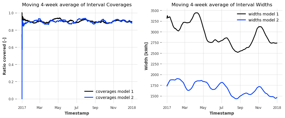
../_images/examples_23-Conformal-Prediction-examples_29_1.png

两个模型的覆盖率随时间稳定，但模型 2 的区间宽度持续较低 -> 我们可以清楚地说模型 2 是赢家（通过较低的不确定性）。

示例 2：多步预测¶

多步预测是开箱即用的。只需设置 n>1（或 forecast_horizon），模型就会为每一步生成校准的预测区间。

[15]:

multi_horizon = 24
pred = cp_model.predict(n=multi_horizon, series=cal, **pred_kwargs)

# plot
ax = series[pred.start_time() - 7 * 24 * series.freq : pred.end_time()].plot(
    label="actual"
)
pred.plot()

[15]:

<Axes: xlabel='Timestamp'>

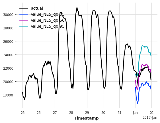
../_images/examples_23-Conformal-Prediction-examples_32_3.png

哦，为什么我们现在有这么大的区间？这是因为我们使用了模型 1（较差的模型），它只训练用来预测下一小时。然后它在内部执行自回归来在校准集上生成 24 小时的预测。因此，预测越远，误差/非一致性分数就越大，最终导致模型不确定性越高。

如果我们使用一个直接训练来预测未来 24 小时的基础预测器，我们可以做得更好。

[16]:

multi_horizon = 24

model = LinearRegressionModel(lags=input_length, output_chunk_length=multi_horizon).fit(
    train
)
cp_model = ConformalNaiveModel(model=model, quantiles=quantiles, cal_length=four_weeks)

pred = cp_model.predict(n=multi_horizon, series=cal, **pred_kwargs)

# plot
ax = series[pred.start_time() - 7 * 24 * series.freq : pred.end_time()].plot(
    label="actual"
)
pred.plot()

[16]:

<Axes: xlabel='Timestamp'>

../_images/examples_23-Conformal-Prediction-examples_34_3.png

示例 3：具有有效覆盖率的定期多步预测¶

但是，如果我们想按计划执行多步预测呢？

例如，我们想每 24 小时进行一次为期一天（24 小时）的预测。

默认情况下，校准集考虑校准集上所有可能的历史预测（cal_stride=1）。这将使用在我们 24 小时计划之外生成的示例，并可能导致无效的覆盖率。

设置 cal_stride=24 将提取正确的示例。

[17]:

# conformal model
cp_model = ConformalNaiveModel(
    model=model,
    quantiles=quantiles,
    cal_length=100,
    cal_stride=multi_horizon,  # stride for calibration set
)

hfcs = cp_model.historical_forecasts(
    series=cal_test,
    forecast_horizon=multi_horizon,
    start=test.start_time(),
    last_points_only=False,  # return each multi-horizon forecast
    stride=multi_horizon,  # use the same stride for historical forecasts
    **pred_kwargs,
)

# concatenate the forecasts into a single TimeSeries
hfcs_concat = concatenate(hfcs, axis=0)
plot_historical_forecasts(hfcs_concat)

bt = cp_model.backtest(
    cal_test,
    historical_forecasts=hfcs,
    last_points_only=False,
    metric=[metrics.mic, metrics.miw],
    metric_kwargs={"q_interval": q_interval},
)
pd.DataFrame({"Interval": q_range, "Coverage": bt[0], "Width": bt[1]})

[17]:

	区间	覆盖率	宽度
0	0.9	0.902283	4772.75975

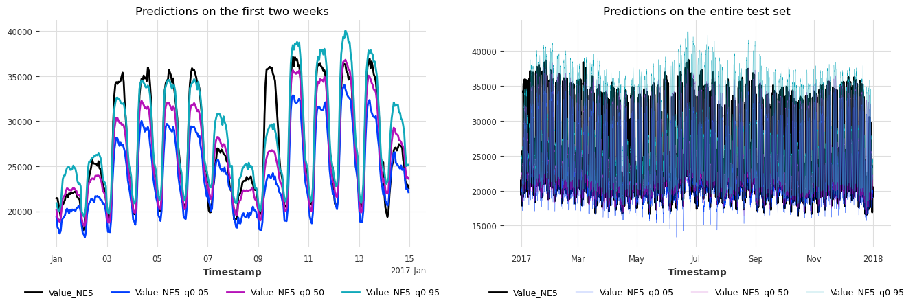
../_images/examples_23-Conformal-Prediction-examples_36_3.png

太棒了，当我们每天只应用一次模型时，我们也实现了有效的覆盖率。

由于我们进行多步预测，检查预测范围内每一步的覆盖率和宽度也很重要。

[18]:

def compute_hfc_horizon_metric(metric=metrics.ic):
    # computes the metric per historical forecast, horizon and component with
    # shape `(n forecasts, horizon, n components, 1)`
    residuals = cp_model.residuals(
        cal_test,
        historical_forecasts=hfcs,
        last_points_only=False,
        metric=metric,
        metric_kwargs={"q_interval": q_interval},
        values_only=True,
    )
    # create array and drop component and sample axes
    residuals = np.array(residuals)[:, :, 0, 0]

    # compute the mean over all forecasts (365 1-day forecasts) for each horizon
    return np.mean(residuals, axis=0)


covs_horizon = compute_hfc_horizon_metric(metrics.ic)
widths_horizon = compute_hfc_horizon_metric(metrics.iw)

[19]:

fig, (ax1, ax2) = plt.subplots(nrows=2, figsize=(6, 8.6), sharex=True)

horizons = [i + 1 for i in range(24)]
ax1.plot(horizons, covs_horizon)
ax2.plot(horizons, widths_horizon)

ax1.set_ylabel("coverage ratio [-]")
ax1.set_title("Interval coverage per step in horizon")

ax2.set_xlabel("horizon")
ax2.set_ylabel("width [kWh]")
ax2.set_title("Interval width per step in horizon");

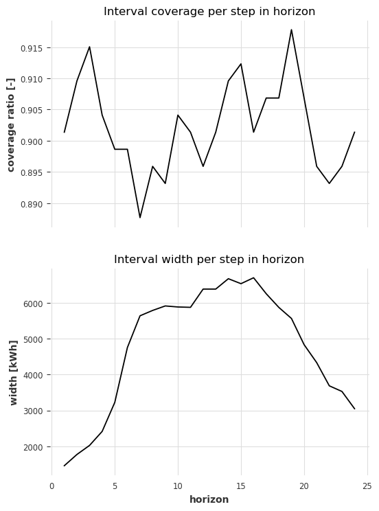
../_images/examples_23-Conformal-Prediction-examples_39_0.png

预测范围内的所有步骤都具有有效覆盖率，范围在 89% 到 92% 之间。

一般来说，宽度随着预测范围的增加而增加。在预测范围 16 之后，它们再次下降，这是由于目标序列的性质（夜间电力消耗较低 -> 不确定性较低）。

示例 4：一致化分位数回归¶

最后，让我们看看 ConformalQRModel 的一个示例。API 完全相同。

唯一的区别是它需要一个概率基础预测器。

让我们使用一个带有分位数回归的线性模型，并执行与示例 1 中相同的单步预测。

[20]:

# probabilistic regression model (with quantiles)
model = LinearRegressionModel(
    lags=input_length,
    output_chunk_length=horizon,
    likelihood="quantile",
    quantiles=quantiles,
).fit(train)

# conformalized quantile regression model
cp_model = ConformalQRModel(model=model, quantiles=quantiles, cal_length=four_weeks)
hfcs = cp_model.historical_forecasts(
    series=cal_test,
    forecast_horizon=horizon,
    start=test.start_time(),
    last_points_only=True,
    stride=horizon,
    **pred_kwargs,
)
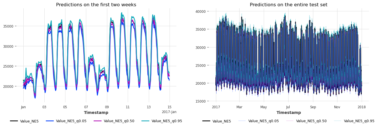
plot_historical_forecasts(hfcs)

bt = cp_model.backtest(
    cal_test,
    historical_forecasts=hfcs,
    last_points_only=True,
    metric=[metrics.mic, metrics.miw],
    metric_kwargs={"q_interval": q_interval},
)
pd.DataFrame({"Interval": q_range, "Coverage": bt[0], "Width": bt[1]})

[20]:

	区间	覆盖率	宽度
0	0.9	0.90024	1770.154514

../_images/examples_23-Conformal-Prediction-examples_42_3.png

覆盖率相同，但区间比朴素一致性预测情况下略大。

回归模型

快速傅里叶变换预测模型 (FFT)