异常检测 Darts 模块
本 notebook 展示了 Darts 异常检测模块的一些功能。我们将了解异常评分器 (Anomaly Scorers)、检测器 (Detectors)、聚合器 (Aggregators) 和异常模型 (Anomaly Models)。
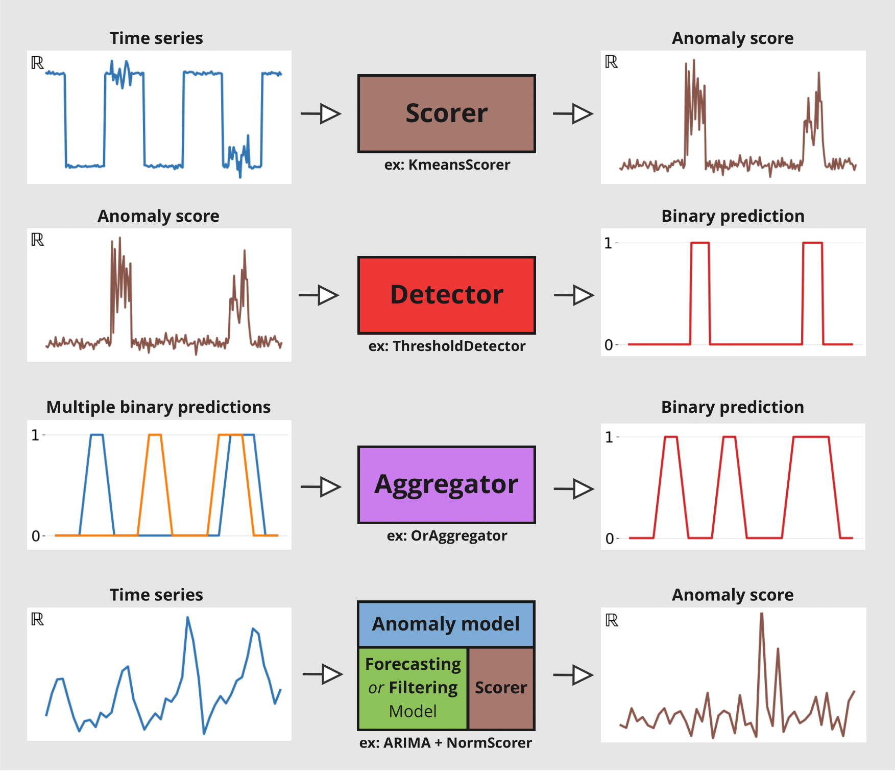
Scorers(评分器):计算异常分数时间序列,既可以在目标序列上计算,也可以在目标序列与预测序列之间计算。它们是异常检测模块的核心。Detectors(检测器):将时间序列(例如异常分数)转换为二元异常时间序列。异常的存在用1标记,否则为0。Aggregators(聚合器):将多变量二元时间序列(例如,每个分量代表不同序列分量/模型的异常分数)简化为单变量二元时间序列。Anomaly Models(异常模型):通过比较模型的预测与实际观测值,提供一种方便的方式来从任何 Darts 全局预测模型或滤波模型生成异常分数。每个异常模型接受一个预测/滤波模型和一个或多个评分器。模型会生成一些预测,这些预测与实际序列一起被馈送到评分器。它将为每个评分器返回异常分数。
下图说明了每个工具的不同输入/输出
本 notebook 分为两个部分
如何使用
ForecastingAnomalyModel在纽约出租车乘客数量中查找异常。如何使用
AnomalyScorer及其窗口功能在两个玩具数据集上的重要性。
首先,进行必要的导入
[1]:
# fix python path if working locally
from utils import fix_pythonpath_if_working_locally

fix_pythonpath_if_working_locally()
%matplotlib inline
[2]:
%load_ext autoreload
%autoreload 2
%matplotlib inline
[3]:
import matplotlib.pyplot as plt
import numpy as np
import pandas as pd

from darts import TimeSeries
from darts.ad import (
    ForecastingAnomalyModel,
    KMeansScorer,
    NormScorer,
    WassersteinScorer,
)
from darts.ad.utils import (
    eval_metric_from_scores,
    show_anomalies_from_scores,
)
from darts.dataprocessing.transformers import Scaler
from darts.datasets import TaxiNewYorkDataset
from darts.metrics import mae, rmse
from darts.models import RegressionModel
/Users/dennisbader/miniconda3/envs/darts310_test/lib/python3.10/site-packages/statsforecast/utils.py:237: FutureWarning: 'M' is deprecated and will be removed in a future version, please use 'ME' instead.
  "ds": pd.date_range(start="1949-01-01", periods=len(AirPassengers), freq="M"),
异常模型:纽约出租车乘客
加载并可视化数据
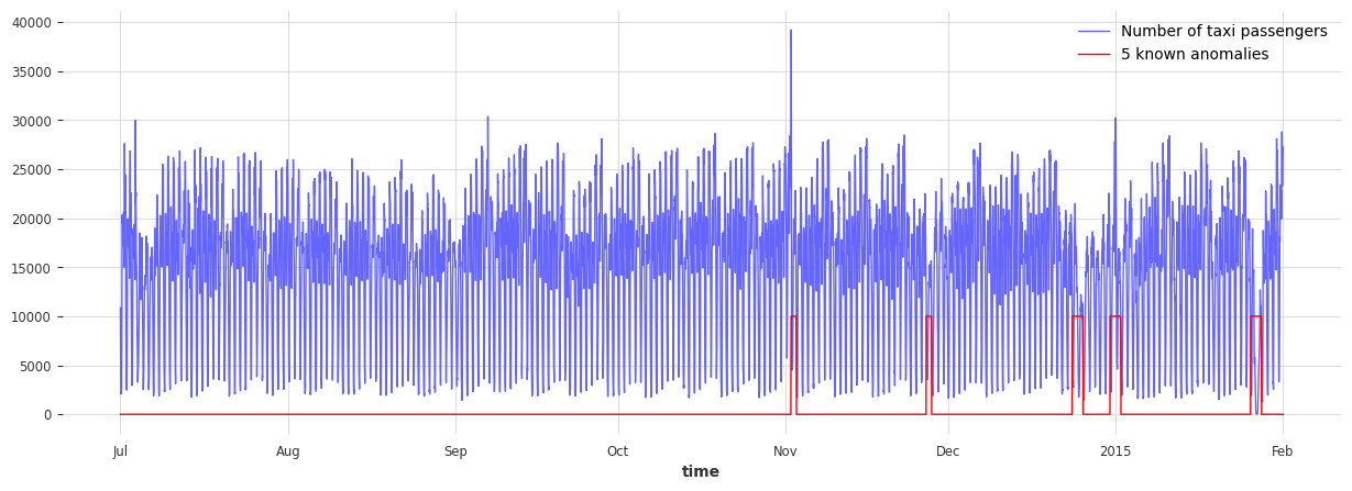
数据信息: - 单变量时间序列(表示纽约出租车乘客数量) - 持续 8 个月(2014 年 7 月至 2015 年 1 月) - 频率为 30 分钟
在此示例中,异常是主观的。它可以定义为出租车需求异常(与预期不同)的时期。基于此定义,以下五个日期可被视为异常
纽约马拉松 - 2014-11-02
感恩节 - 2014-11-27
圣诞节 - 2014-12-24/25
元旦 - 2015-01-01
暴风雪 - 2015-01-26/27
[4]:
# load the data
series_taxi = TaxiNewYorkDataset().load()

# define start and end dates for some known anomalies
anomalies_day = {
    "NYC Marathon": ("2014-11-02 00:00", "2014-11-02 23:30"),
    "Thanksgiving ": ("2014-11-27 00:00", "2014-11-27 23:30"),
    "Christmas": ("2014-12-24 00:00", "2014-12-25 23:30"),
    "New Years": ("2014-12-31 00:00", "2015-01-01 23:30"),
    "Snow Blizzard": ("2015-01-26 00:00", "2015-01-27 23:30"),
}
anomalies_day = {
    k: (pd.Timestamp(v[0]), pd.Timestamp(v[1])) for k, v in anomalies_day.items()
}

# create a series with the binary anomaly flags
anomalies = pd.Series([0] * len(series_taxi), index=series_taxi.time_index)
for start, end in anomalies_day.values():
    anomalies.loc[(start <= anomalies.index) & (anomalies.index <= end)] = 1.0

series_taxi_anomalies = TimeSeries.from_series(anomalies)

# plot the data and the anomalies
fig, ax = plt.subplots(figsize=(15, 5))
series_taxi.plot(label="Number of taxi passengers", linewidth=1, color="#6464ff")
(series_taxi_anomalies * 10000).plot(label="5 known anomalies", color="r", linewidth=1)
plt.show()
[5]:
def plot_anom(selected_anomaly, delta_plotted_days):
    one_day = series_taxi.freq * 24 * 2
    anomaly_date = anomalies_day[selected_anomaly][0]
    start_timestamp = anomaly_date - delta_plotted_days * one_day
    end_timestamp = anomaly_date + (delta_plotted_days + 1) * one_day

    series_taxi[start_timestamp:end_timestamp].plot(
        label="Number of taxi passengers", color="#6464ff", linewidth=0.8
    )

    (series_taxi_anomalies[start_timestamp:end_timestamp] * 10000).plot(
        label="Known anomaly", color="r", linewidth=0.8
    )
    plt.title(selected_anomaly)
    plt.show()


for anom_name in anomalies_day:
    plot_anom(anom_name, 3)
    break  # remove this to see all anomalies
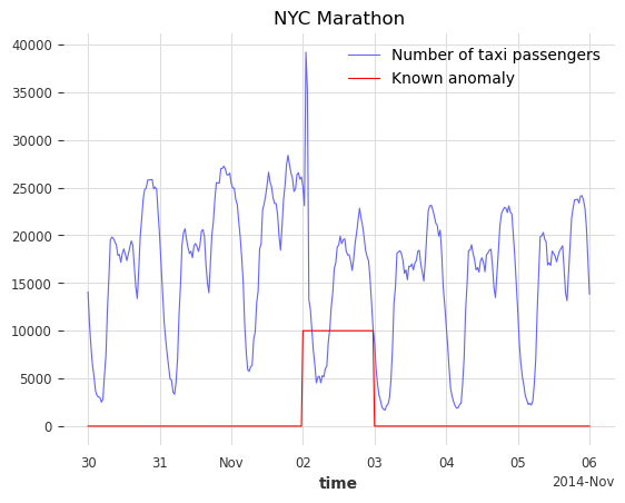
目标是检测这五个不规律的时期,并识别其他可能的异常日期。
训练 Darts 预测模型
我们将使用 RegressionModel 来预测出租车乘客数量。前 4500 个时间戳将用于训练模型。训练集被认为是无异常的,所考虑的五个异常位于第 4500 个时间戳之后。滞后数设置为 1 周,假设需求遵循 1 周的周期性。为了帮助模型,有关目标序列的附加信息(小时和星期几)作为协变量传递。
[6]:
# split the data in a training and testing set
s_taxi_train = series_taxi[:4500]
s_taxi_test = series_taxi[4500:]

# Add covariates (hour and day of the week)
add_encoders = {
    "cyclic": {"future": ["hour", "dayofweek"]},
}

# one week corresponds to (7 days * 24 hours * 2) of 30 minutes
one_week = 7 * 24 * 2

forecasting_model = RegressionModel(
    lags=one_week,
    lags_future_covariates=[0],
    output_chunk_length=1,
    add_encoders=add_encoders,
)
forecasting_model.fit(s_taxi_train)
[6]:
RegressionModel(lags=336, lags_past_covariates=None, lags_future_covariates=[0], output_chunk_length=1, output_chunk_shift=0, add_encoders={'cyclic': {'future': ['hour', 'dayofweek']}}, model=None, multi_models=True, use_static_covariates=True)
使用预测异常模型
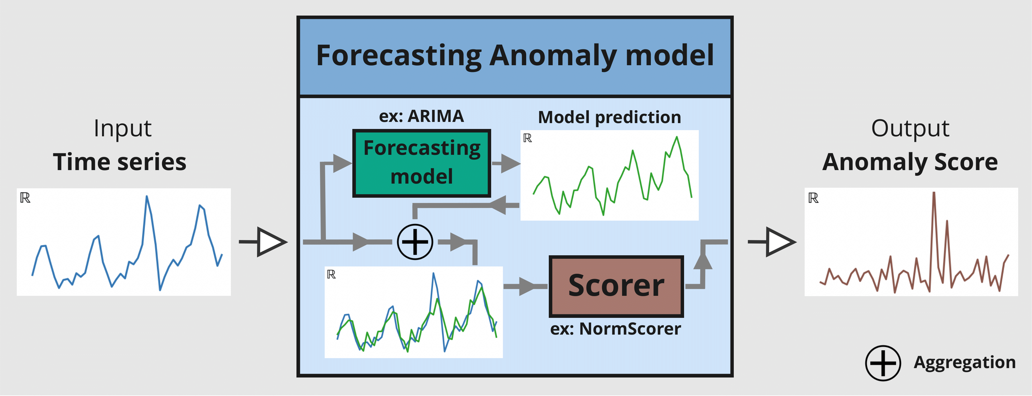
异常模型包含两个输入: - 一个已拟合的 GlobalForecastingModel(列表可见此处。如果模型尚未拟合,请在调用 fit() 时将参数 allow_model_training 设置为 True) - 一个或多个 AnomalyScorer(可训练或不可训练)
在此示例中,将使用三个评分器: - NormScorer(窗口默认为 1) - WassersteinScorer,使用半天窗口(24 个时间戳)且无窗口聚合 - WassersteinScorer,使用全天窗口(48 个时间戳)并包含窗口聚合
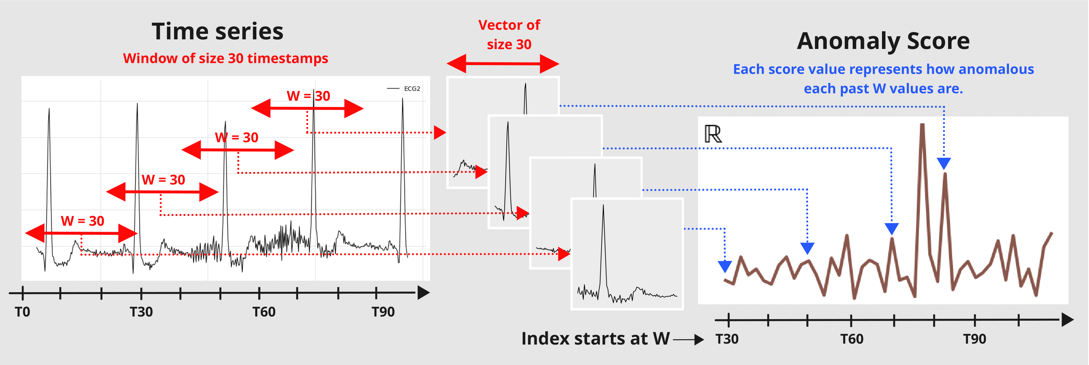
参数 window 是一个整数值,表示评分器用于将序列转换为异常分数时使用的窗口大小。评分器会将给定序列切片成大小为 W 的子序列,并返回一个值,指示这些大小为 W 的子集值的异常程度。
可以使用 window_agg 通过聚合包含该点的每个窗口中的所有异常分数,将窗口级别分数转换为点级别分数。
下图说明了预测异常模型的机制
使用主要函数: fit() 、 score() 、 eval_metric() 和 show_anomalies() 
[7]:
# with timestamps of 30 minutes
half_a_day = 2 * 12
full_day = 2 * 24

# instantiate the anomaly model with: one fitted model, and 3 scorers
anomaly_model = ForecastingAnomalyModel(
    model=forecasting_model,
    scorer=[
        NormScorer(ord=1),
        WassersteinScorer(window=half_a_day, window_agg=False),
        WassersteinScorer(window=full_day, window_agg=True),
    ],
)
现在让我们使用 fit() 训练异常模型。它将按顺序执行以下操作
如果预测模型尚未拟合且
allow_model_training=True,则在给定序列上拟合预测模型。为给定序列生成历史预测。
将历史预测馈送到每个可拟合/可训练的评分器
计算预测与给定序列之间的差异(由评分器的
diff_fn控制,参见 Darts “每时间步” 指标此处)在这些差异上训练评分器
您可以在调用 fit() 时控制如何生成历史预测(支持的参数参见此处)。
[8]:
START = 0.1
anomaly_model.fit(s_taxi_train, start=START, allow_model_training=False, verbose=True)
[8]:
<darts.ad.anomaly_model.forecasting_am.ForecastingAnomalyModel at 0x2905d0130>
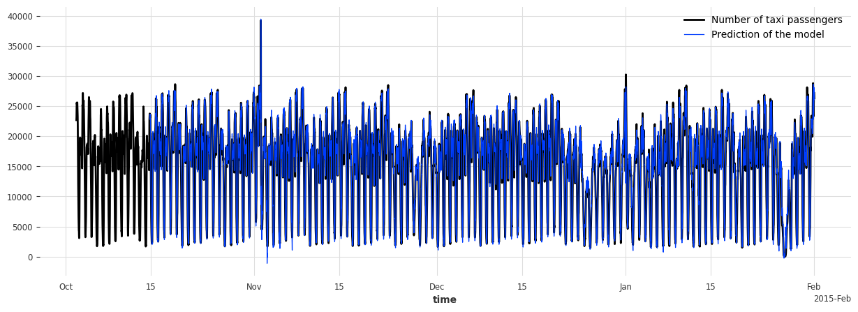
我们调用函数 score() 来计算新序列 s_taxi_test 的异常分数。它返回异常模型中每个评分器的分数。我们将在下一节使用这些结果。通过设置 return_model_prediction=True,我们还可以额外获取预测模型生成的历史预测。
[9]:
anomaly_scores, model_forecasting = anomaly_model.score(
    s_taxi_test, start=START, return_model_prediction=True, verbose=True
)
pred_start = model_forecasting.start_time()
[10]:
# compute the MAE and RMSE on the test set
print(
    f"On testing set -> MAE: {mae(model_forecasting, s_taxi_test)}, RMSE: {rmse(model_forecasting, s_taxi_test)}"
)

# plot the data and the anomalies
fig, ax = plt.subplots(figsize=(15, 5))
s_taxi_test.plot(label="Number of taxi passengers")
model_forecasting.plot(label="Prediction of the model", linewidth=0.9)
plt.show()
On testing set -> MAE: 595.190366262045, RMSE: 896.6287614972252
为了评估异常模型,我们调用函数 eval_metric()。它输出预测异常分数时间序列与指示实际异常存在的已知二元地面真值时间序列之间的无关阈值指标(“AUC-ROC” 或 “AUC-PR”)的分数。
它将返回一个包含评分器名称及其分数的字典。
[11]:
metric_names = ["AUC_ROC", "AUC_PR"]
metric_data = []
for metric_name in metric_names:
    metric_data.append(
        anomaly_model.eval_metric(
            anomalies=series_taxi_anomalies,
            series=s_taxi_test,
            start=START,
            metric=metric_name,
        )
    )
pd.DataFrame(data=metric_data, index=metric_names).T
[11]:
| AUC_ROC | AUC_PR | |
|---|---|---|
| 范数 (ord=1)_w=1 | 0.658074 | 0.215601 |
| WassersteinScorer_w=24 | 0.884915 | 0.609469 |
| WassersteinScorer_w=48 | 0.950035 | 0.687788 |
我们可以看到,使用 WassersteinScorer 的异常模型能够将异常日期与正常日期区分开。AUC ROC 高于 0.9。此外,大小为 48 个时间戳(24 小时)的窗口比大小为 24 个时间戳(12 小时)的窗口是更好的选择。
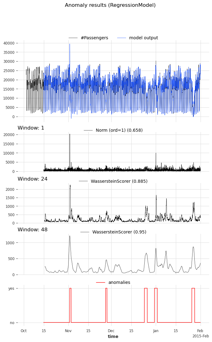
我们调用函数 show_anomalies() 来可视化结果。它会绘制预测、预测分数、输入序列以及实际异常(如果提供)。不同窗口的评分器将分开显示。可以计算一个指标,并显示在评分器名称旁边。
[12]:
anomaly_model.show_anomalies(
    series=s_taxi_test,
    anomalies=series_taxi_anomalies[pred_start:],
    start=START,
    metric="AUC_ROC",
)
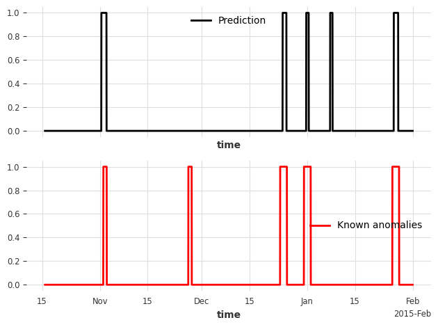
使用 Detector 将异常分数转换为二元预测
Darts 的异常检测器将异常分数转换为二元异常/预测。在此示例中,我们将使用 QuantileDetector。
它根据历史数据的分位数 (high_quantile 和/或 low_quantile) 来检测异常。当值超过这些分位数阈值时,它将时间标记为异常。在此示例中,异常分数是针对模型的绝对残差计算的。它的下界是 0。我们将 low_quantile 设置为 None(默认),因为我们只想标记高于 high_quantile 的值。
我们将 high_quantile 设置为 0.95。必须仔细选择此值,因为它会将 (1- high_quantile) * 100 % 的最大异常分数转换为异常预测。在我们的示例中,我们希望看到 5% 最异常的时间戳。
注意:您还可以使用
ThresholdDetector定义一些固定的值阈值进行异常检测
[13]:
from darts.ad.detectors import QuantileDetector

contamination = 0.95
detector = QuantileDetector(high_quantile=contamination)
[14]:
# use the anomaly score that gave the best AUC ROC score: Wasserstein anomaly score with a window of 'full_day'
best_anomaly_score = anomaly_scores[-1]

# fit and detect on the anomaly scores, it will return a binary prediction
anomaly_pred = detector.fit_detect(series=best_anomaly_score)

# plot the binary prediction
fig, (ax1, ax2) = plt.subplots(nrows=2, sharex=True)
anomaly_pred.plot(label="Prediction", ax=ax1)
series_taxi_anomalies[anomaly_pred.start_time() :].plot(
    label="Known anomalies", ax=ax2, color="red"
)
fig.tight_layout()
[15]:
for metric_name in ["accuracy", "precision", "recall", "f1"]:
    metric_val = detector.eval_metric(
        pred_scores=best_anomaly_score,
        anomalies=series_taxi_anomalies,
        window=full_day,
        metric=metric_name,
    )
    print(metric_name + f": {metric_val:.2f}/1")
accuracy: 0.91/1
precision: 0.76/1
recall: 0.32/1
f1: 0.45/1
在内部,方法 eval_metric() 和 show_anomalies() 分别调用 eval_metric_from_scores() 和 show_anomalies_from_scores()。我们也可以直接使用预先计算的异常分数调用它们,以避免每次都重新生成分数。
让我们重现以上结果。这两个函数都需要用于计算每个异常分数的窗口大小。在我们的示例中,窗口大小分别为 1, 24 (half_a_day), 48 (full_day)。
[16]:
windows = [1, half_a_day, full_day]
scorer_names = [f"{scorer}_{w}" for scorer, w in zip(anomaly_model.scorers, windows)]

metric_data = {"AUC_ROC": [], "AUC_PR": []}
for metric_name in metric_data:
    metric_data[metric_name] = eval_metric_from_scores(
        anomalies=series_taxi_anomalies,
        pred_scores=anomaly_scores,
        window=windows,
        metric=metric_name,
    )

pd.DataFrame(index=scorer_names, data=metric_data)
[16]:
| AUC_ROC | AUC_PR | |
|---|---|---|
| 范数 (ord=1)_1 | 0.658074 | 0.215601 |
| WassersteinScorer_24 | 0.884915 | 0.609469 |
| WassersteinScorer_48 | 0.950035 | 0.687788 |
正如所料,AUC ROC 和 AUC PR 值与之前相同。
用于可视化异常
如果我们想计算一个指标,也需要指定窗口大小
可选地,我们可以指示生成分数的评分器名称
[17]:
show_anomalies_from_scores(
    series=s_taxi_test,
    anomalies=series_taxi_anomalies[pred_start:],
    pred_scores=anomaly_scores,
    pred_series=model_forecasting,
    window=windows,
    title="Anomaly results using a forecasting method",
    names_of_scorers=scorer_names,
    metric="AUC_ROC",
)

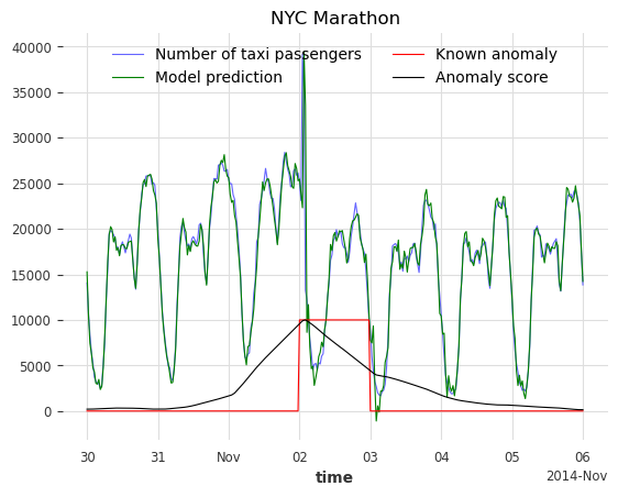
放大查看各异常:可视化结果
[18]:
def plot_anom_eval(selected_anomaly, delta_plotted_days):
    one_day = series_taxi.freq * 24 * 2
    anomaly_date = anomalies_day[selected_anomaly][0]
    start = anomaly_date - one_day * delta_plotted_days
    end = anomaly_date + one_day * (delta_plotted_days + 1)

    # input series and forecasts
    series_taxi[start:end].plot(
        label="Number of taxi passengers", color="#6464ff", linewidth=0.8
    )
    model_forecasting[start:end].plot(
        label="Model prediction", color="green", linewidth=0.8
    )

    # actual anomalies and predicted scores
    (series_taxi_anomalies[start:end] * 10000).plot(
        label="Known anomaly", color="r", linewidth=0.8
    )
    # Scaler transforms scores into a value range between (0, 1)
    (Scaler().fit_transform(best_anomaly_score)[start:end] * 10000).plot(
        label="Anomaly score", color="black", linewidth=0.8
    )
    plt.legend(loc="upper center", ncols=2)
    plt.title(selected_anomaly)
    fig.tight_layout()
    plt.show()


for anom_name in anomalies_day:
    plot_anom_eval(anom_name, 3)
    break  # remove this to see all anomalies
简单示例: KMeansScorer 
让我们以 KmeansScorer 为例,仔细看看评分器的 window 参数。我们将使用两个玩具数据集来演示评分器在不同窗口大小下的表现。在第一个示例中,我们将 window 设置为 1 处理多变量时间序列,在第二个示例中,我们将 window 设置为 2 处理单变量时间序列。
下图说明了评分器的窗口处理过程
多变量情况,窗口大小 window=1
合成数据创建
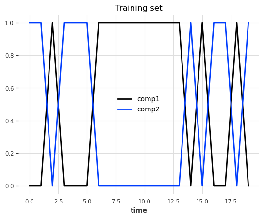
数据是一个多变量序列(2 个分量/列)。每一步的值要么是 0 要么是 1,并且两个分量的值总是相反的
[19]:
pd.DataFrame(index=["State 1", "State 2"], data={"comp1": [0, 1], "comp2": [1, 0]})
[19]:
| 分量 1 | 分量 2 | |
|---|---|---|
| 状态 1 | 0 | 1 |
| 状态 2 | 1 | 0 |
在每个时间戳,有 50% 的机会切换状态,有 50% 的机会保持相同状态。
训练集
[20]:
def generate_data_ex1(random_state: int):
    np.random.seed(random_state)

    # create the train set
    comp1 = np.expand_dims(np.random.choice(a=[0, 1], size=100, p=[0.5, 0.5]), axis=1)
    comp2 = (comp1 == 0).astype(float)
    vals = np.concatenate([comp1, comp2], axis=1)
    return vals
[21]:
data = generate_data_ex1(random_state=40)
series_train = TimeSeries.from_values(data, columns=["comp1", "comp2"])

# visualize the train set
series_train[:20].plot()
plt.title("Training set")
plt.show()
测试集
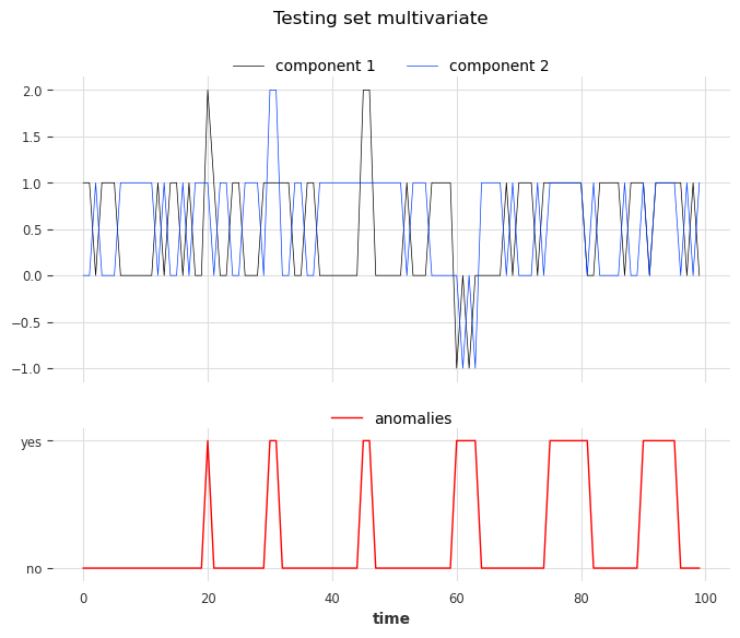
我们使用与训练集相同的规则创建测试集,但将注入六个不同类型的异常。异常可以长于一个时间戳。类型如下:
第 1 类:将一个分量的值(0 或 1)替换为 2
第 2 类:给两个分量都加上 +1 或 -1
第 3 类:两个分量具有相同的值
[22]:
# inject anomalies in the test timeseries
data = generate_data_ex1(random_state=3)

# 2 anomalies per type
# type 1: random values for only one component
data[20:21, 0] = 2
data[30:32, 1] = 2

# type 2: shift both components values (+/- 1 for both components)
data[45:47, :] += 1
data[60:64, :] -= 1

# type 3: switch one value to the another
data[75:82, 0] = data[75:82, 1]
data[90:96, 1] = data[90:96, 0]

series_test = TimeSeries.from_values(data, columns=["component 1", "component 2"])

# create the binary anomalies ground truth series
anomalies = ~((data == [0, 1]).all(axis=1) | (data == [1, 0]).all(axis=1))
anomalies = TimeSeries.from_times_and_values(
    times=series_test.time_index, values=anomalies, columns=["is_anomaly"]
)
让我们看看这些异常。从左到右,前两个异常对应第一类,第三个和第四个对应第二类,最后两个对应第三类。
[23]:
show_anomalies_from_scores(
    series=series_test, anomalies=anomalies, title="Testing set multivariate"
)
使用评分器 KMeansScorer() 
我们将使用 KMeansScorer 并使用以下参数定位异常
k=2:KMeans 模型生成的聚类/质心数量。我们选择两个,因为我们知道只有两种有效状态。window=1(默认):KMeans 模型独立考虑每个时间戳。它表示用于创建序列子序列的窗口大小(对于我们的回归模型,window等同于正向目标lag)。在此示例中,我们知道仅查看一步就可以检测到每个异常。component_wise=False(默认):所有分量与单个 KMeans 模型一起用作特征。如果为True,我们将为每个分量拟合一个专用模型。在此示例中,我们需要有关两个分量的信息来查找所有异常。
我们将在无异常的训练序列上拟合 KMeansScorer,在测试序列上计算异常分数,最后评估分数。
[24]:
Kmeans_scorer = KMeansScorer(k=2, window=1, component_wise=False)

# fit the KmeansScorer on the train timeseries 'series_train'
Kmeans_scorer.fit(series_train)
[24]:
<darts.ad.scorers.kmeans_scorer.KMeansScorer at 0x29a3849d0>
[25]:
anomaly_score = Kmeans_scorer.score(series_test)

# visualize the anomaly score compared to the true anomalies
anomaly_score.plot(label="Anomaly score by KMeans")
(anomalies - 2).plot()
plt.title("Anomaly score from KMeans Scorer vs true anomalies")
plt.show()
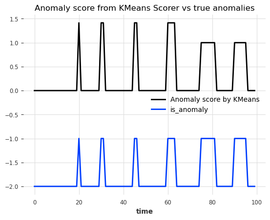
很好!我们可以看到异常分数准确地指示了 6 个异常的位置。
要评估分数,我们可以调用 eval_metric()。它需要真实异常、序列以及无关阈值指标(AUC-ROC 或 AUC-PR)的名称。
[26]:
for metric_name in ["AUC_ROC", "AUC_PR"]:
    metric_val = Kmeans_scorer.eval_metric(anomalies, series_test, metric=metric_name)
    print(metric_name + f": {metric_val}")
AUC_ROC: 1.0
AUC_PR: 1.0
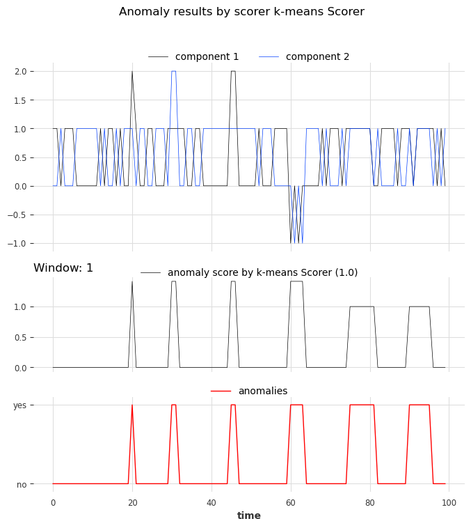
再来,让我们使用 show_anomalies() 可视化结果
[27]:
Kmeans_scorer.show_anomalies(series=series_test, anomalies=anomalies, metric="AUC_ROC")
单变量情况,窗口大小 window>1
在前面的示例中,我们使用了 window=1,这足以识别所有异常。在下一个示例中,我们将看到有时需要更大的值才能捕获真实异常。
合成数据创建
训练集
在这个玩具示例中,我们生成一个单变量(一个分量)序列,它可以取 4 个可能的值。
每一步的可能值
(0, 1, 2, 3)下一步要么加上
diff=+1,要么减去diff=-1(50% 概率)所有步都有上下界
0和diff=-1保持在03和diff=+1保持在3
[28]:
def generate_data_ex2(start_val: int, random_state: int):
    np.random.seed(random_state)
    # create the test set
    vals = np.zeros(100)

    vals[0] = start_val

    diffs = np.random.choice(a=[-1, 1], p=[0.5, 0.5], size=len(vals) - 1)
    for i in range(1, len(vals)):
        vals[i] = vals[i - 1] + diffs[i - 1]
        if vals[i] > 3:
            vals[i] = 3
        elif vals[i] < 0:
            vals[i] = 0
    return vals
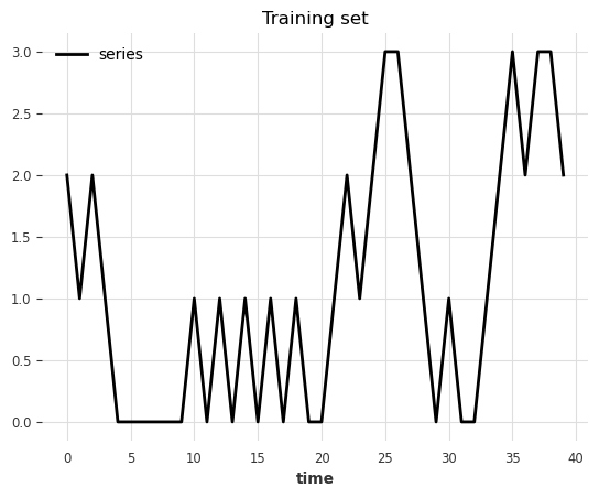
[29]:
data = generate_data_ex2(start_val=2, random_state=1)
series_train = TimeSeries.from_values(data, columns=["series"])

# visualize the train set
series_train[:40].plot()
plt.title("Training set")
[29]:
Text(0.5, 1.0, 'Training set')
测试集
我们使用与训练集相同的规则创建测试集,但将注入六个不同类型的异常。异常可以长于一个时间戳
类型 1:步长
abs(diff) > 1(跳跃大于 1)类型 2:在值
(1, 2)时diff = 0(值保持不变)
[30]:
data = generate_data_ex2(start_val=1, random_state=3)

# 3 anomalies per type
# type 1: sudden shift between state 0 to state 2 without passing by value 1
data[23] = 3
data[44] = 3
data[91] = 0

# type 2: having consecutive timestamps at value 1 or 2
data[3:5] = 2
data[17:19] = 1
data[62:65] = 2

series_test = TimeSeries.from_values(data, columns=["series"])

# identify the anomalies
diffs = np.abs(data[1:] - data[:-1])
anomalies = ~((diffs == 1) | ((diffs == 0) & np.isin(data[1:], [0, 3])))
# the first step is not an anomaly
anomalies = np.concatenate([[False], anomalies]).astype(int)

anomalies = TimeSeries.from_times_and_values(
    series_test.time_index, anomalies, columns=["is_anomaly"]
)
[31]:
show_anomalies_from_scores(
    series=series_test, anomalies=anomalies, title="Testing set univariate"
)
plt.show()
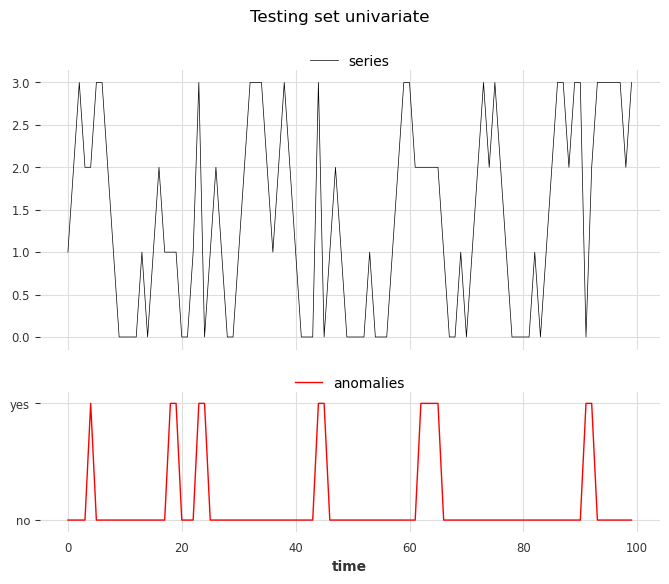
从左到右,位置 3、4 和 6 的异常属于类型 1,位置 1、2 和 5 的异常属于类型 2。
使用评分器 KMeansScorer() 
我们拟合了两个 KMeansScorer,对 window 参数使用不同的值(1 和 2)。
[32]:
windows = [1, 2]
Kmeans_scorer_w1 = KMeansScorer(k=4, window=windows[0])
Kmeans_scorer_w2 = KMeansScorer(k=8, window=windows[1], window_agg=False)
[33]:
scores_all = []
metric_data = {"AUC_ROC": [], "AUC_PR": []}
for model, window in zip([Kmeans_scorer_w1, Kmeans_scorer_w2], windows):
    model.fit(series_train)
    scores = model.score(series_test)
    scores_all.append(scores)

    for metric_name in metric_data:
        metric_data[metric_name].append(
            eval_metric_from_scores(
                anomalies=anomalies,
                pred_scores=scores,
                metric=metric_name,
            )
        )
pd.DataFrame(data=metric_data, index=["w_1", "w_2"])
[33]:
| AUC_ROC | AUC_PR | |
|---|---|---|
| w_1 | 0.460212 | 0.123077 |
| w_2 | 1.000000 | 1.000000 |
该指标表明,参数窗口设置为 1 的评分器无法定位异常。另一方面,参数设置为 2 的评分器完美地识别了异常。
[34]:
show_anomalies_from_scores(
    series=series_test,
    anomalies=anomalies,
    pred_scores=scores_all,
    names_of_scorers=["KMeansScorer_w1", "KMeansScorer_w2"],
    metric="AUC_ROC",
    title="Anomaly results from KMeansScorer",
)
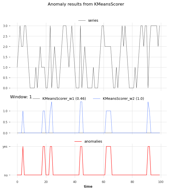
我们可以看到窗口大小为 2 的评分器的预测比窗口大小为 1 的评分器更准确。
[ ]: