动态时间规整 (DTW)
以下演示了 darts 中 DTW 模块的功能。动态时间规整允许您比较长度和时间轴不同的两个时间序列。该算法将确定两个序列中元素之间的最佳对齐方式,以最小化它们之间的成对距离。
[1]:
# fix python path if working locally
from utils import fix_pythonpath_if_working_locally

fix_pythonpath_if_working_locally()
[2]:
%load_ext autoreload
%autoreload 2
%matplotlib inline

import numpy as np
import pandas as pd
from matplotlib import pyplot as plt
from scipy.signal import argrelextrema

from darts.dataprocessing import dtw
from darts.datasets import SunspotsDataset
from darts.metrics import dtw_metric, mae
from darts.models import MovingAverageFilter
from darts.timeseries import TimeSeries
[3]:
SMALL_SIZE = 30
MEDIUM_SIZE = 35
BIGGER_SIZE = 40
FIG_WIDTH = 20
FIG_SIZE = (40, 10)


plt.rc("font", size=SMALL_SIZE)  # controls default text sizes
plt.rc("axes", titlesize=SMALL_SIZE)  # fontsize of the axes title
plt.rc("axes", labelsize=MEDIUM_SIZE)  # fontsize of the x and y labels
plt.rc("xtick", labelsize=SMALL_SIZE)  # fontsize of the tick labels
plt.rc("ytick", labelsize=SMALL_SIZE)  # fontsize of the tick labels
plt.rc("legend", fontsize=SMALL_SIZE)  # legend fontsize
plt.rc("figure", titlesize=BIGGER_SIZE)  # fontsize of the figure title
plt.rc("figure", figsize=FIG_SIZE)  # size of the figure
读取和格式化
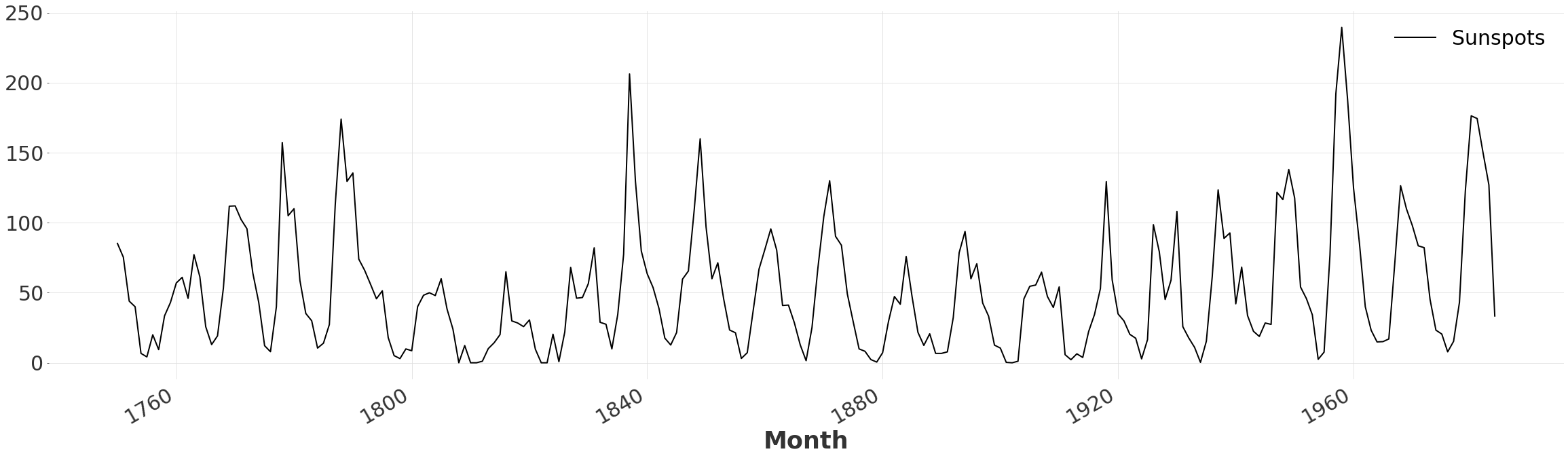
在这里,我们只是简单地读取包含太阳黑子数量的 CSV 文件,并将值转换为所需的格式。我们对数据集进行重采样以消除高频噪声,因为我们只关注其总体形状。
[4]:
ts = SunspotsDataset().load()
ts = ts.resample(freq="y")
ts.plot()
确定峰值数量
我们观察到该序列由一系列尖锐的峰和谷组成。让我们快速确定需要考虑的周期数。我们首先对序列应用移动平均滤波器,以消除虚假的局部最大值。然后我们只需计数由 argrelextrema 返回的局部最大值数量。
[5]:
ts_smooth = MovingAverageFilter(window=3).filter(ts)

minimums = argrelextrema(ts_smooth.univariate_values(), np.greater)

periods = len(minimums[0])
periods
[5]:
24
生成用于比较的模式
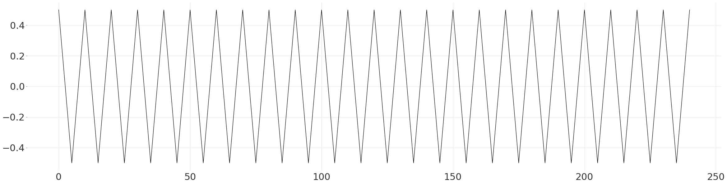
在这里,我们根据先前的观察,简单地构建一个由线性峰和谷组成的简化模式。我们确保其均值为 0 且范围为 1,以便更容易拟合到数据。
[6]:
steps = int(np.ceil(len(ts) / (periods * 2)))
down = np.linspace(0.5, -0.5, steps + 1)[:-1]
up = np.linspace(-0.5, 0.5, steps + 1)[:-1]

values = np.append(np.tile(np.append(down, up), periods), 0.5)

plt.plot(np.arange(len(values)), values)
将模式拟合到序列
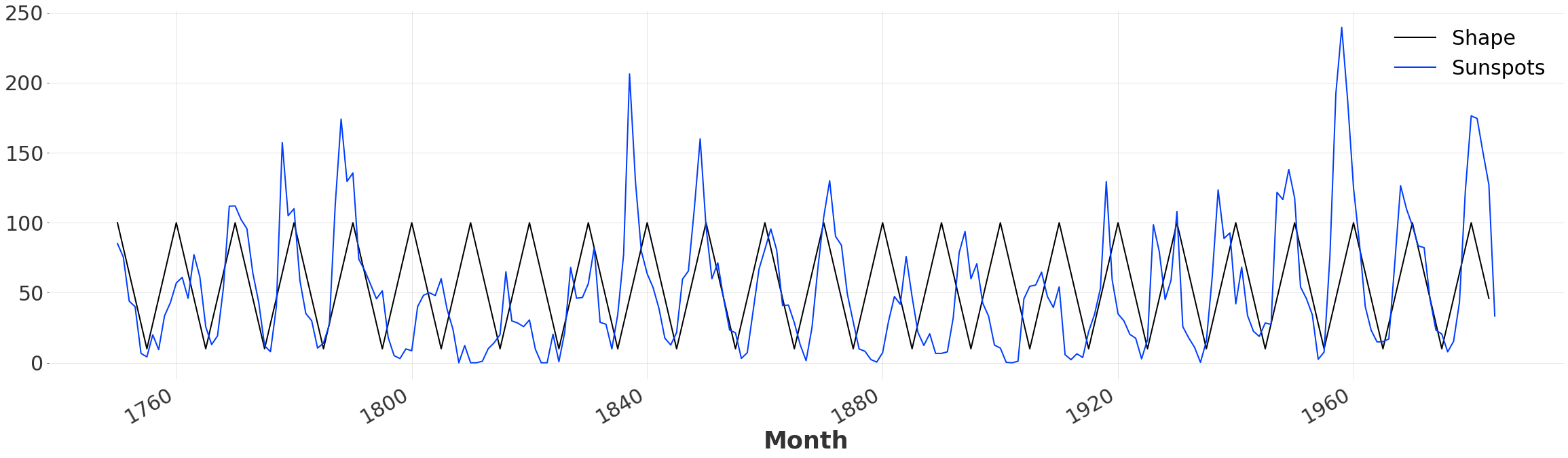
我们对数据进行重新缩放和偏移,使其与实际序列对齐。然后我们创建一个新的 TimeSeries,其时间轴与太阳黑子数据集相同。虽然这不是执行动态时间规整所必需的,但这将使我们能够绘制和比较初始对齐结果。由于我们的模式略长于太阳黑子时间序列本身,我们丢弃了截止日期之后的所有值。
[7]:
m = 90
c = 55

scaled_values = values * m + c

time_range = pd.date_range(start=ts.start_time(), freq="y", periods=len(values))
ts_shape_series = pd.Series(scaled_values, index=time_range, name="Shape")

ts_shape = TimeSeries.from_series(ts_shape_series)
ts_shape = ts_shape.drop_after(ts.end_time())
ts_shape.plot()
ts.plot()
定量比较
我们可以使用平均绝对误差(也称为 mae)来评估我们的简单模式与数据拟合的紧密程度。从上面的图表可以看出,峰值之间的时间存在一些波动,这导致了未对齐和相对较高的误差。
[8]:
original_mae = mae(ts, ts_shape)
original_mae
[8]:
34.01837606837607
进入动态时间规整
幸运的是,查找两个序列之间的最佳对齐正是 DTW 的设计目的!我们只需调用 dtw 并传入两个时间序列即可。
无窗口
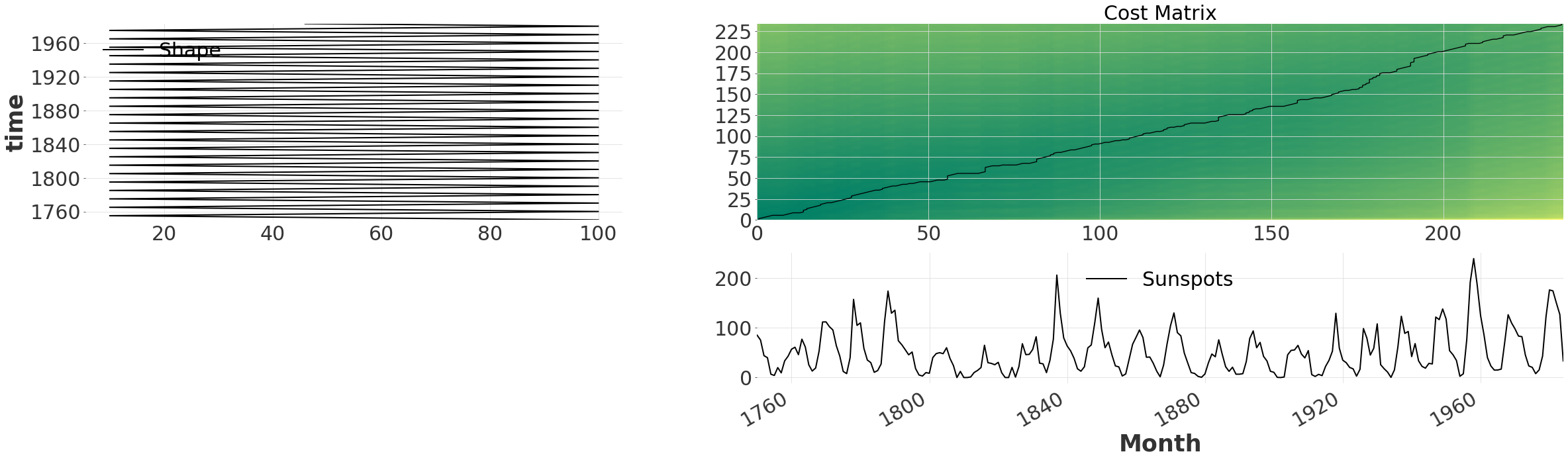
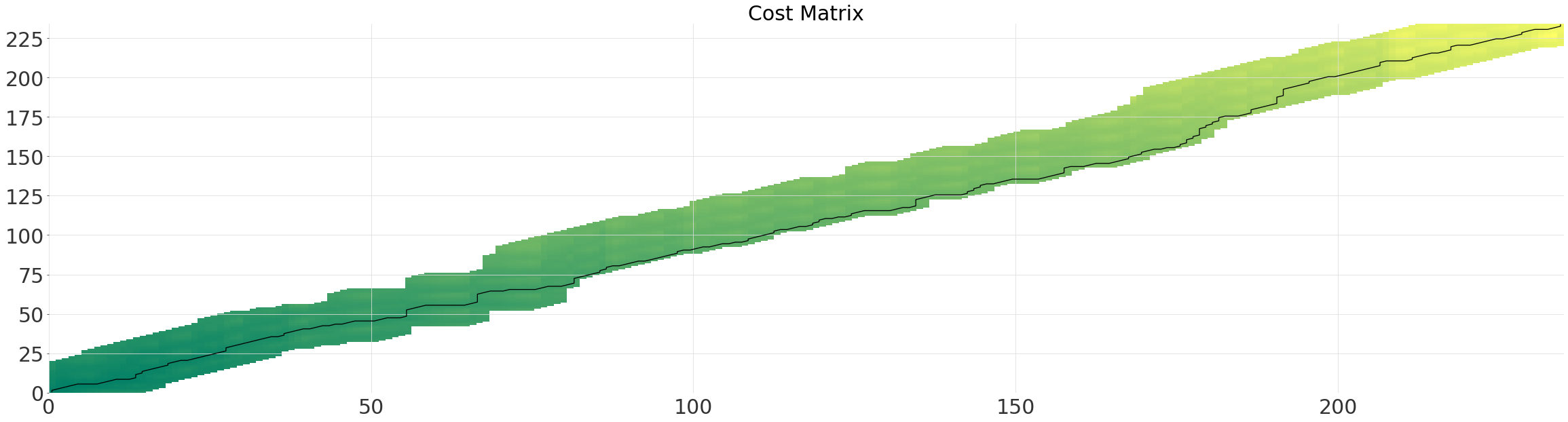
默认行为是考虑时间序列之间所有可能的对齐方式。当我们使用 .plot() 绘制成本矩阵及其路径时,这一点变得很明显。成本矩阵表示将 (i,j) 匹配在一起的对齐的总成本/距离。对于我们的时间序列,我们观察到一条深绿色带穿过对角线。这表明两个时间序列在开始时大部分已经对齐。
[9]:
exact_alignment = dtw.dtw(ts, ts_shape)
exact_alignment.plot(show_series=True)
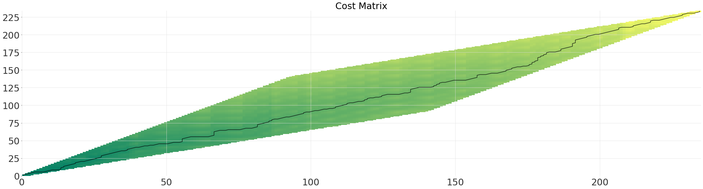
多网格
在大型数据集上计算所有可能的对齐方式会很快变得计算成本高昂(平方复杂度)。
相反,我们可以使用多网格求解器,它以接近线性时间运行。求解器首先在较小的网格上确定最佳路径,然后递归地重新投影和细化路径,每次将分辨率加倍。简单地启用多网格求解器(线性复杂度)通常会带来巨大的速度提升,而不会损失太多精度。
参数 multi_grid_radius 控制从较低分辨率下找到的路径扩展搜索窗口的程度。换句话说,增加它会以性能为代价来提高精度。
[10]:
multi_grid_radius = 10

multigrid_alignment = dtw.dtw(ts, ts_shape, multi_grid_radius=multi_grid_radius)
multigrid_alignment.plot()
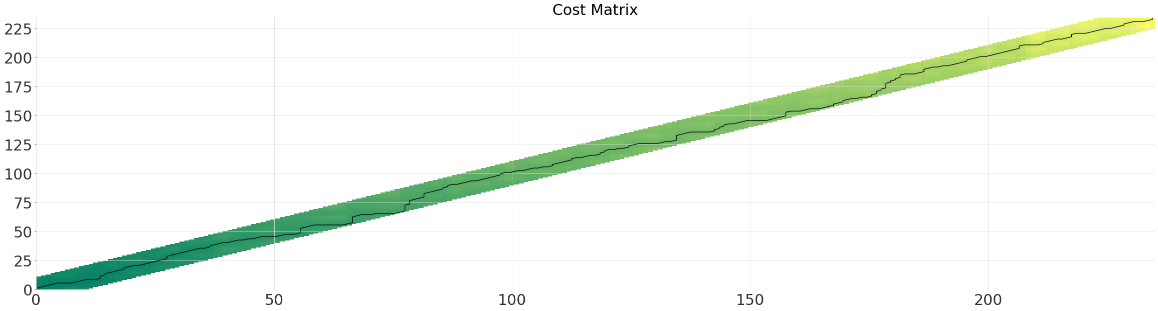
对角窗口 (SakoeChiba)
SakoeChiba 窗口形成一个对角带,其范围由参数 window_size 确定。当您知道两个时间序列大部分已经对齐或想要限制规整量时,此窗口最适用。它将确保一个序列中的元素 n,只与另一个序列中与 n 索引差在 window_size 范围内的元素匹配。
[11]:
sakoechiba_alignment = dtw.dtw(ts, ts_shape, window=dtw.SakoeChiba(window_size=10))
sakoechiba_alignment.plot()
平行四边形窗口 (Itakura)
参数 max_slope 控制平行四边形较陡一侧的斜率。对于我们的时间序列,该窗口有点浪费,因为最优路径并未显著偏离对角线。
[12]:
itakura_alignment = dtw.dtw(ts, ts_shape, window=dtw.Itakura(max_slope=1.5))
itakura_alignment.plot()
不同对齐方式的比较
尽管每种窗口都会导致不同的运行时,但路径的长度实际上是相同的。如果我们进一步约束窗口或减小 multi_grid_radius,我们将发现最优路径会比其他路径更短。
[13]:
alignments = [
    exact_alignment,
    multigrid_alignment,
    sakoechiba_alignment,
    itakura_alignment,
]
names = ["Exact (Optimal)", "Multi-Grid", "Sakoe-Chiba", "Itakura"]
distances = [align.distance() for align in alignments]

plt.title("Absolute DTW Distance (Lower is Better)")
plt.bar(names, distances)

alignment = multigrid_alignment
可视化对齐结果
[14]:
alignment.plot_alignment(series2_y_offset=200)
plt.gca().set_title("Warp Alignment")

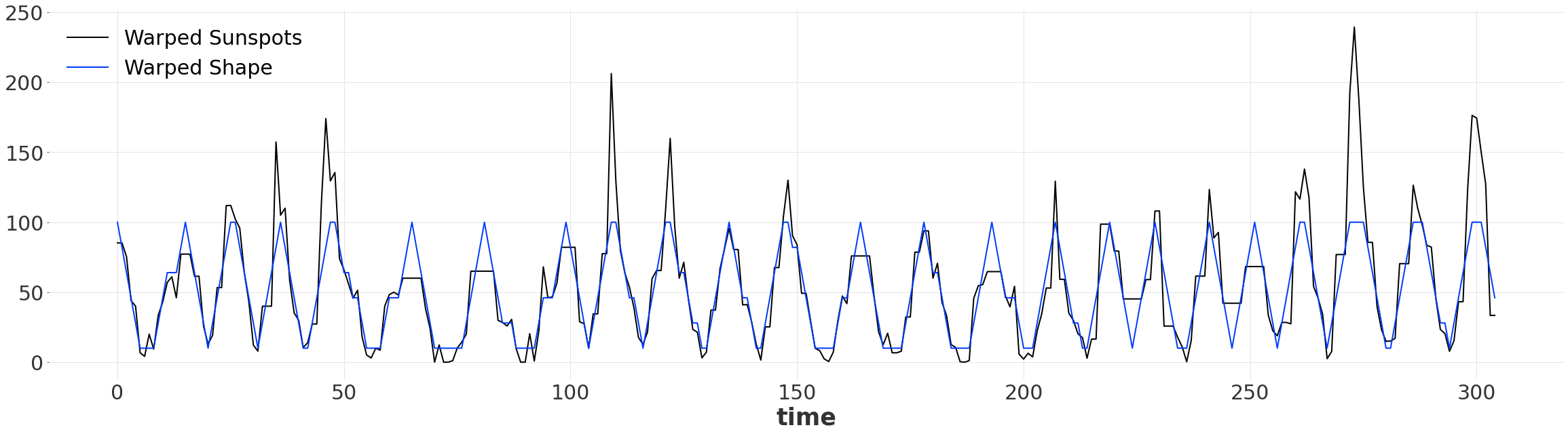
规整后的时间序列
一旦找到对齐方式,我们就可以生成两个长度相同的规整序列。由于我们对时间维度进行了规整,默认情况下,新的规整序列使用 pd.RangeIndex 进行索引。现在,我们的简单模式与序列匹配,尽管它们最初并不匹配!
[15]:
warped_ts, warped_ts_shape = alignment.warped()

warped_ts.plot(label="Warped Sunspots")
warped_ts_shape.plot(label="Warped Shape")
定量比较
我们可以再次应用 mae 指标,但这次是对规整后的序列。如果我们只对规整后的相似性感兴趣,我们也可以直接调用辅助函数 dtw_metric。注意到规整后序列之间的误差减少了约 65%!
[16]:
warped_mae0 = mae(warped_ts, warped_ts_shape)
warped_mae1 = dtw_metric(ts, ts_shape, metric=mae, multi_grid_radius=multi_grid_radius)

plt.bar(["Original", "Warped", "DTW Metric"], [original_mae, warped_mae0, warped_mae1])

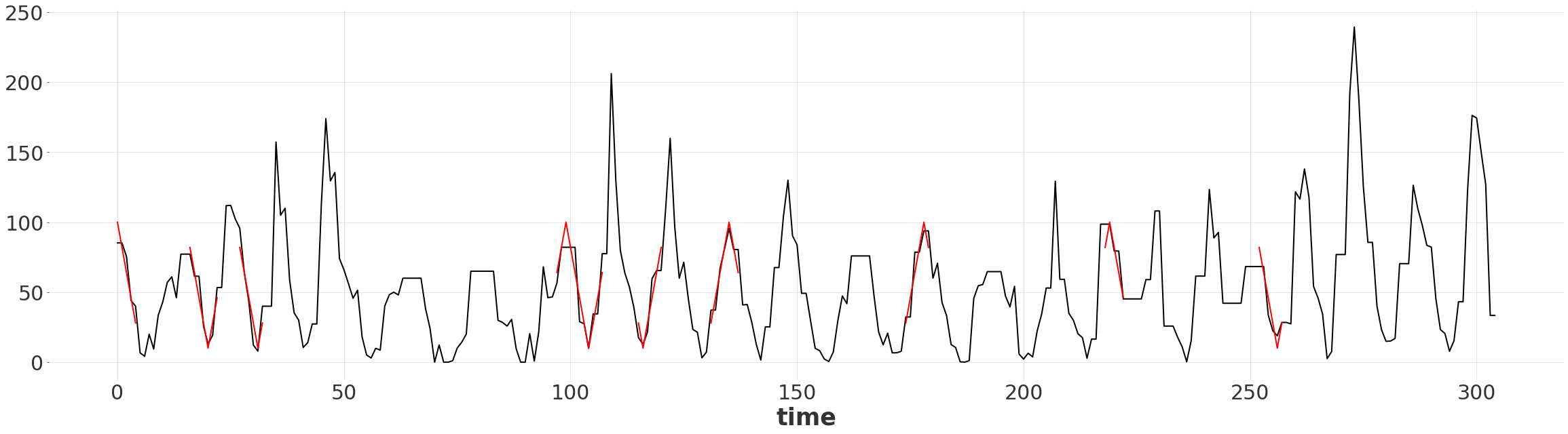
查找匹配的子序列
给定对齐方式,我们可以找到两个时间序列的匹配子序列。
两个元素之间的差值小于某个阈值
原始模式未被扭曲
子序列具有某个最小长度
[17]:
THRESHOLD = 20
MATCH_MIN_LENGTH = 5

path = alignment.path()
path = path.reshape((-1,))

warped_ts_values = warped_ts.univariate_values()
warped_ts_shape_values = warped_ts_shape.univariate_values()

within_threshold = (
    np.abs(warped_ts_values - warped_ts_shape_values) < THRESHOLD
)  # Criterion 1
linear_match = np.diff(path[1::2]) == 1  # Criterion 2

matches = np.logical_and(within_threshold, np.append(True, linear_match))
if not matches[-1]:
    matches = np.append(matches, False)

matched_ranges = []
match_begin = 0

last_m = False
for i, m in enumerate(matches):
    if last_m and not m:
        match_end = i - 1
        match_len = match_end - match_begin

        if match_len >= MATCH_MIN_LENGTH:  # Criterion 3
            matched_ranges.append(pd.RangeIndex(match_begin, i - 1))
    if not last_m and m:
        match_begin = i
    last_m = m

matched_ranges
[17]:
[RangeIndex(start=0, stop=5, step=1),
 RangeIndex(start=16, stop=23, step=1),
 RangeIndex(start=27, stop=33, step=1),
 RangeIndex(start=97, stop=108, step=1),
 RangeIndex(start=115, stop=121, step=1),
 RangeIndex(start=131, stop=138, step=1),
 RangeIndex(start=174, stop=180, step=1),
 RangeIndex(start=218, stop=223, step=1),
 RangeIndex(start=252, stop=258, step=1)]
可视化匹配的子序列
我们可以简单地通过 RangeIndex 对规整后的形状序列进行切片,以提取子序列。
[18]:
warped_ts.plot()

for r in matched_ranges:
    warped_ts_shape[r].plot(color="red")

plt.gca().get_legend().remove()
[ ]: