使用 darts 滤波器进行滤波和预测

在此 notebook 中，我们将探讨卡尔曼滤波算法如何用于提高受噪声影响的数据质量。白噪声是任何类型传感器采集数据中的常见成分。

卡尔曼滤波器是 Darts 中一种不同类型的模型，它是一个 FilteringModel（而不是 ForecastingModel），可用于平滑序列。对于卡尔曼滤波器，观测值的“实际”底层值是使用线性动力系统的状态空间模型推断出来的。该系统可以作为输入提供，也可以在数据上进行拟合。

在此 notebook 中，我们将生成一个简单的合成数据集，并看看卡尔曼滤波器如何用于去噪。请注意，这只是一个玩具示例，主要是为了展示 Darts 卡尔曼滤波器 API 的工作原理。

%reload_ext autoreload
%autoreload 2
%matplotlib inline

import matplotlib.pyplot as plt
import numpy as np

from darts import TimeSeries
from darts.models import KalmanFilter
from darts.utils import timeseries_generation as tg

一阶系统的阶跃响应

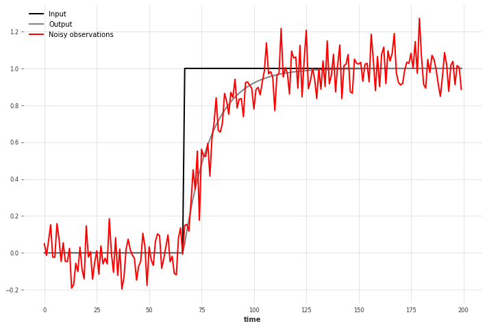
测量中常见的信号形状是指数趋于稳态的形状，例如在系统收敛到设定点时。我们首先准备输入（控制信号）和输出，并添加噪声以获得逼真的观测值。

NOISE_DISTANCE = 0.1
SAMPLE_SIZE = 200
np.random.seed(42)

# Prepare the input
u = TimeSeries.from_values(np.heaviside(np.linspace(-5, 10, SAMPLE_SIZE), 0))

# Prepare the output
y = u * TimeSeries.from_values(1 - np.exp(-np.linspace(-5, 10, SAMPLE_SIZE)))

# Add white noise to obtain the observations
noise = tg.gaussian_timeseries(length=SAMPLE_SIZE, std=NOISE_DISTANCE)
y_noise = y + noise

plt.figure(figsize=[12, 8])
u.plot(label="Input")
y.plot(color="gray", label="Output")
y_noise.plot(color="red", label="Noisy observations")
plt.legend()
plt.show()

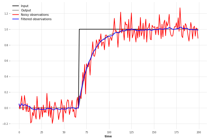
这种行为可以通过一阶线性动力系统建模，使其成为 dim_x=1 的卡尔曼滤波器的理想选择。

我们使用输入作为协变量拟合卡尔曼滤波器，并对相同的时间序列进行滤波。请注意，如果我们在更长的时间序列上拟合模型，结果可能会更好。

滤波后的观测值相当接近无噪声的输出信号，并且在输入发生阶跃变化时尤其能很好地跟踪输出。这与移动平均等滤波方法不同，这表明模型确实考虑了输入（协变量）。

我们可以观察到时间序列开始时的误差较大，因为卡尔曼滤波器在该点几乎没有信息来估计状态。

kf = KalmanFilter(dim_x=1)
kf.fit(y_noise, u)
y_filtered = kf.filter(y_noise, u)

plt.figure(figsize=[12, 8])
u.plot(label="Input")
y.plot(color="gray", label="Output")
y_noise.plot(color="red", label="Noisy observations")
y_filtered.plot(color="blue", label="Filtered observations")
plt.legend()

<matplotlib.legend.Legend at 0x7fc594431ed0>

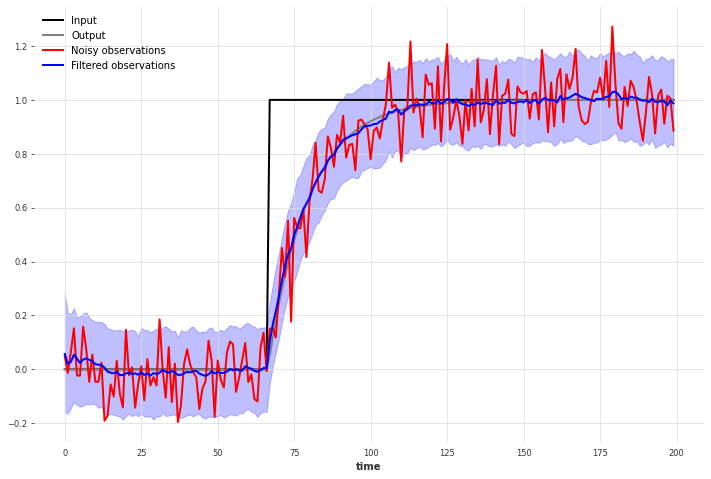
我们还可以通过增加 num_samples 来获得底层值的概率估计。

y_filtered = kf.filter(y_noise, u, num_samples=1000)

plt.figure(figsize=[12, 8])
u.plot(label="Input")
y.plot(color="gray", label="Output")
y_noise.plot(color="red", label="Noisy observations")
y_filtered.plot(color="blue", label="Filtered observations")
plt.legend()

<matplotlib.legend.Legend at 0x7fc581075190>

螺旋绘图

首先，让我们绘制一个简单的图形并添加明显的白噪声。

NOISE_DISTANCE = 0.5
SAMPLE_SIZE = 10000
RESIZE_NOISE = 150

# Prepare the drawing
theta = np.radians(np.linspace(360 * 15, 0, SAMPLE_SIZE))
r = theta**2
x_2 = r * np.cos(theta)
y_2 = r * np.sin(theta)

# add white noise (gaussian noise, can be mapped from the random distribution using rand**3)
# and resize to RESIZE_NOISE
x_2_noise = x_2 + (np.random.normal(0, NOISE_DISTANCE, SAMPLE_SIZE) ** 3) * RESIZE_NOISE
y_2_noise = y_2 + (np.random.normal(0, NOISE_DISTANCE, SAMPLE_SIZE) ** 3) * RESIZE_NOISE

plt.figure(figsize=[20, 20])
plt.plot(x_2_noise, y_2_noise, color="red", label="Noisy spiral drawing.")
plt.plot(x_2, y_2, label="Original spiral drawing.")
plt.legend()
plt.show()

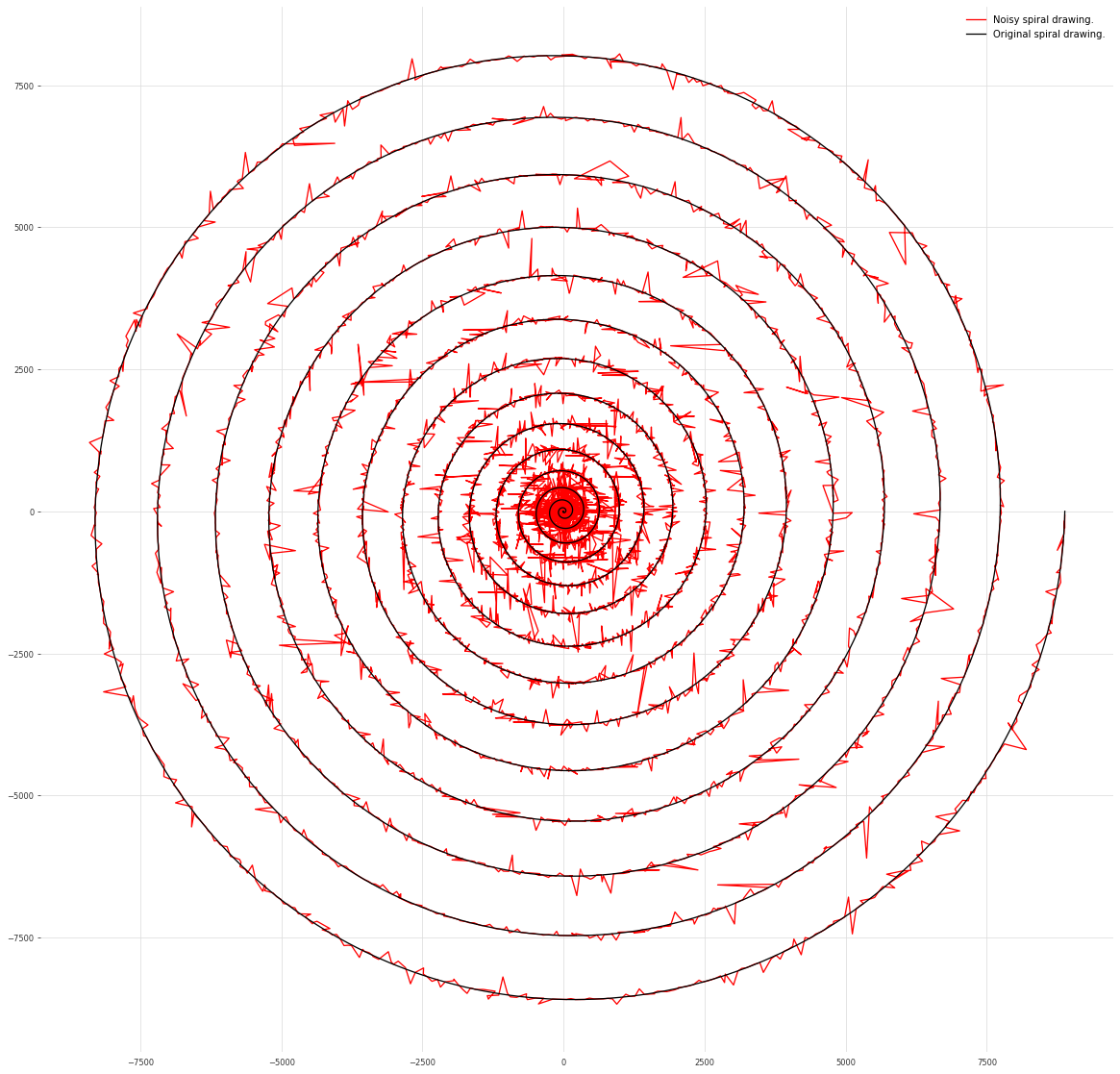
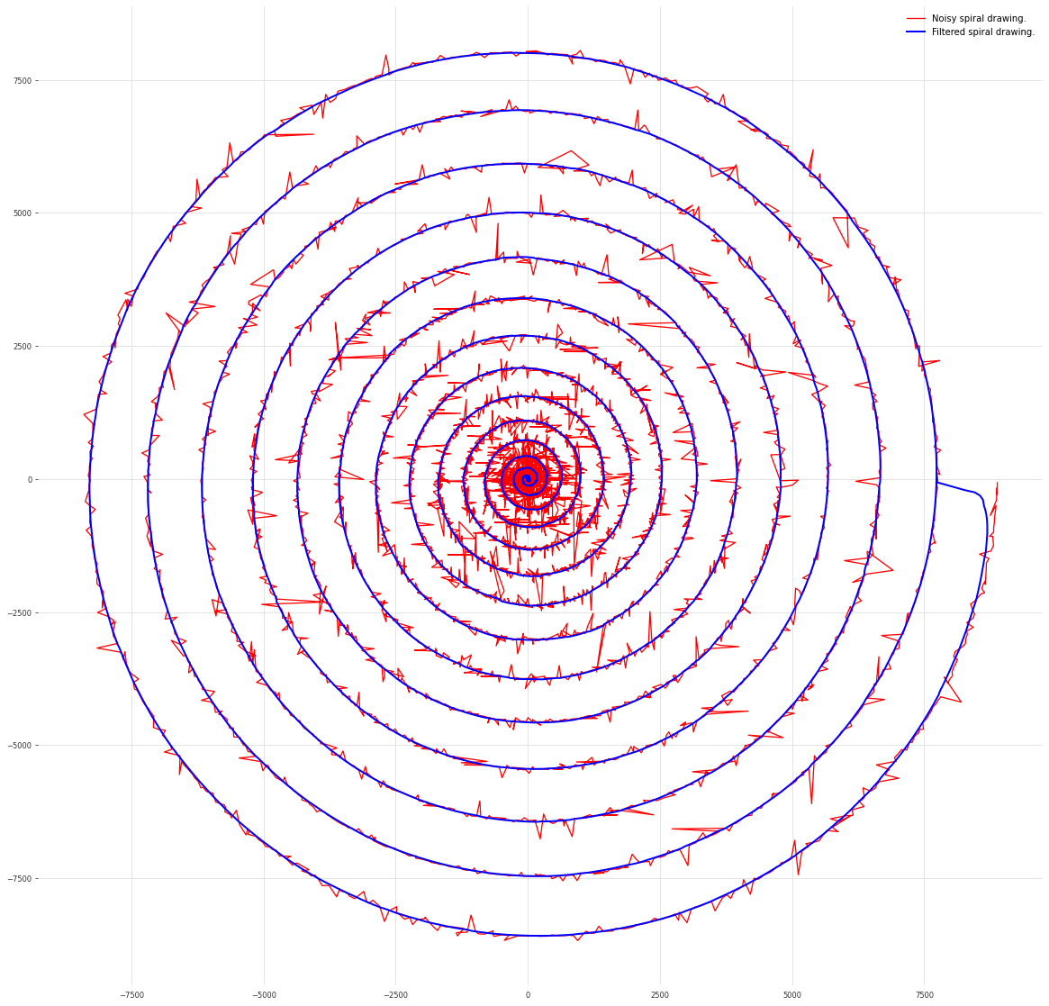
上述图形可以使用没有输入（衰减到其平衡点 (0, 0)）的二阶线性动力系统生成。因此，我们可以使用 dim_x=2 的卡尔曼滤波器对包含“x”和“y”分量的多元时间序列进行拟合。我们看到卡尔曼滤波器在螺旋绘图去噪方面做得很好。

请注意，我们必须调整参数 num_block_rows 以使模型拟合收敛。

kf = KalmanFilter(dim_x=2)
ts = TimeSeries.from_values(x_2_noise).stack(TimeSeries.from_values(y_2_noise))
kf.fit(ts, num_block_rows=50)

filtered_ts = kf.filter(ts).values()
filtered_x = filtered_ts[:, 0]
filtered_y = filtered_ts[:, 1]

plt.figure(figsize=[20, 20])
plt.plot(x_2_noise, y_2_noise, color="red", label="Noisy spiral drawing.")
plt.plot(
    filtered_x, filtered_y, color="blue", linewidth=2, label="Filtered spiral drawing."
)
plt.legend()

<matplotlib.legend.Legend at 0x7fc58144a950>

上一篇

集成模型

下一篇

使用高斯过程滤波器进行滤波和预测