使用 Darts 进行时间序列预测的迁移学习

作者：Julien Herzen, Florian Ravasi, Guillaume Raille, Gaël Grosch。

概述

本 notebook 的目标是探索时间序列预测中的迁移学习——即在一个时间序列数据集上训练预测模型，并将其应用于另一个数据集。本 notebook 是完全独立的——也就是说，它包含了安装依赖项和下载所用数据集所需的命令。

根据构成“学习任务”的不同，我们在此处所说的迁移学习也可以从元学习（或“学会学习”）的角度来看待，在这种学习中，模型可以在推理时适应新任务（例如，预测新的时间序列），而无需进一步训练 [1]。

本 notebook 改编自 2022 年 3 月在瑞士洛桑举行的应用机器学习日大会上关于“预测与元学习”的研讨会。它包含以下几个部分：

• 第 0 部分：初始设置 - 导入、数据下载函数等。

• 第 1 部分：预测 300 家航空公司的乘客数量序列（air 数据集）。我们将为每个序列训练一个模型。

• 第 2 部分：使用“全局”模型 - 即同时在所有 300 个序列上训练的模型。

• 第 3 部分：我们将尝试一些迁移学习，看看如果在某个（大数据）数据集（m4 数据集）上训练一些全局模型，并将其应用于另一个数据集时会发生什么。

• 第 4 部分：我们将把第 3 部分的预训练模型重复用于另一个新数据集（m3 数据集），并比较其与专门在此数据集上训练的模型的效果。

不同模型的计算时长是通过在搭载 Apple Silicon M2 CPU、使用 Python 3.10.13 和 Darts 0.27.0 的环境下运行本 notebook 获得的。

第 0 部分：设置

首先，我们需要安装正确的库并进行正确的导入。对于深度学习模型来说，有 GPU 会有帮助，但这并非强制要求。

以下两个单元格只需要运行一次。它们用于安装依赖项并下载所有必要的数据集。

!pip install xlrd
!pip install darts

# Execute this cell once to download all three datasets
!curl -L https://forecasters.org/data/m3comp/M3C.xls -o m3_dataset.xls
!curl -L https://data.transportation.gov/api/views/xgub-n9bw/rows.csv -o carrier_passengers.csv
!curl -L https://raw.githubusercontent.com/Mcompetitions/M4-methods/master/Dataset/Train/Monthly-train.csv \
    -o m4_monthly.csv
!curl -L https://raw.githubusercontent.com/Mcompetitions/M4-methods/master/Dataset/M4-info.csv -o m4_metadata.csv

  % Total    % Received % Xferd  Average Speed   Time    Time     Time  Current
                                 Dload  Upload   Total   Spent    Left  Speed
100 1716k  100 1716k    0     0  6899k      0 --:--:-- --:--:-- --:--:-- 6949k
  % Total    % Received % Xferd  Average Speed   Time    Time     Time  Current
                                 Dload  Upload   Total   Spent    Left  Speed
100 56.3M    0 56.3M    0     0  1747k      0 --:--:--  0:00:33 --:--:-- 2142k
  % Total    % Received % Xferd  Average Speed   Time    Time     Time  Current
                                 Dload  Upload   Total   Spent    Left  Speed
100 87.4M  100 87.4M    0     0  26.2M      0  0:00:03  0:00:03 --:--:-- 26.3M
  % Total    % Received % Xferd  Average Speed   Time    Time     Time  Current
                                 Dload  Upload   Total   Spent    Left  Speed
100 4233k  100 4233k    0     0  5150k      0 --:--:-- --:--:-- --:--:-- 5163k      0      0 --:--:-- --:--:-- --:--:--     0

现在我们导入所有内容。别担心，我们将通过本 notebook 揭示这些导入的含义 :)

%matplotlib inline

import warnings

warnings.filterwarnings("ignore")


import random
import time
from datetime import datetime
from itertools import product
from typing import Optional

import matplotlib.pyplot as plt
import numpy as np
import pandas as pd
import torch
from sklearn.preprocessing import MaxAbsScaler
from tqdm.auto import tqdm

from darts import TimeSeries
from darts.dataprocessing.transformers import Scaler
from darts.metrics import smape
from darts.models import (
    ARIMA,
    ExponentialSmoothing,
    KalmanForecaster,
    LightGBMModel,
    LinearRegressionModel,
    NaiveSeasonal,
    NBEATSModel,
    RandomForest,
    Theta,
)
from darts.utils.losses import SmapeLoss

我们在这里定义预测范围 - 对于本 notebook 中使用的所有（月度）时间序列，我们将对提前 18 个月进行预测感兴趣。我们选择 18 个月是因为这是 M3/M4 竞赛中对月度序列使用的范围。

HORIZON = 18

数据集加载方法

在这里，我们定义了一些辅助方法来加载我们将使用的三个数据集：air、m3 和 m4。

下面所有方法都返回两个 TimeSeries 列表：一个训练序列列表和一个“测试”序列列表（长度为 HORIZON）。

为了方便起见，所有序列在这里都已缩放，通过将每个序列乘以一个常数，使其最大值为 1。这种缩放对于许多模型（特别是深度学习模型）正常工作是必要的。它不影响 sMAPE 值，因此我们可以在缩放后的序列上评估算法的准确性。在实际应用中，我们需要将 Darts Scaler 对象保存在某个地方以便对预测结果进行反向缩放。

如果您有兴趣查看如何创建和缩放 TimeSeries 的示例，可以查看 load_m3() 函数。

def load_m3() -> tuple[list[TimeSeries], list[TimeSeries]]:
    print("building M3 TimeSeries...")

    # Read DataFrame
    df_m3 = pd.read_excel("m3_dataset.xls", "M3Month")

    # Build TimeSeries
    m3_series = []
    for row in tqdm(df_m3.iterrows()):
        s = row[1]
        start_year = int(s["Starting Year"])
        start_month = int(s["Starting Month"])
        values_series = s[6:].dropna()
        if start_month == 0:
            continue

        start_date = datetime(year=start_year, month=start_month, day=1)
        time_axis = pd.date_range(start_date, periods=len(values_series), freq="M")
        series = TimeSeries.from_times_and_values(
            time_axis, values_series.values
        ).astype(np.float32)
        m3_series.append(series)

    print(f"\nThere are {len(m3_series)} monthly series in the M3 dataset")

    # Split train/test
    print("splitting train/test...")
    m3_train = [s[:-HORIZON] for s in m3_series]
    m3_test = [s[-HORIZON:] for s in m3_series]

    # Scale so that the largest value is 1
    print("scaling...")
    scaler_m3 = Scaler(scaler=MaxAbsScaler())
    m3_train_scaled: list[TimeSeries] = scaler_m3.fit_transform(m3_train)
    m3_test_scaled: list[TimeSeries] = scaler_m3.transform(m3_test)

    print(
        f"done. There are {len(m3_train_scaled)} series, with average training length {np.mean([len(s) for s in m3_train_scaled])}"  # noqa: E501
    )
    return m3_train_scaled, m3_test_scaled


def load_air() -> tuple[list[TimeSeries], list[TimeSeries]]:
    # download csv file
    df = pd.read_csv("carrier_passengers.csv")
    # extract relevant columns
    df = df[["data_dte", "carrier", "Total"]]
    # aggregate per carrier and date
    df = pd.DataFrame(df.groupby(["carrier", "data_dte"]).sum())
    # move indexes to columns
    df = df.reset_index()

    # group bt carrier, specify time index and target variable
    all_air_series = TimeSeries.from_group_dataframe(
        df, group_cols="carrier", time_col="data_dte", value_cols="Total", freq="MS"
    )

    # Split train/test
    print("splitting train/test...")
    air_train = []
    air_test = []
    for series in all_air_series:
        # remove the end of the series
        series = series[: pd.Timestamp("2019-12-31")]
        # convert to proper type
        series = series.astype(np.float32)
        # extract longest contiguous slice
        try:
            series = series.longest_contiguous_slice()
        except Exception:
            continue
        # remove static covariates
        series = series.with_static_covariates(None)
        # remove short series
        if len(series) >= 36 + HORIZON:
            air_train.append(series[:-HORIZON])
            air_test.append(series[-HORIZON:])

    # Scale so that the largest value is 1
    print("scaling series...")
    scaler_air = Scaler(scaler=MaxAbsScaler())
    air_train_scaled: list[TimeSeries] = scaler_air.fit_transform(air_train)
    air_test_scaled: list[TimeSeries] = scaler_air.transform(air_test)

    print(
        f"done. There are {len(air_train_scaled)} series, with average training length {np.mean([len(s) for s in air_train_scaled])}"  # noqa: E501
    )
    return air_train_scaled, air_test_scaled


def load_m4(
    max_number_series: Optional[int] = None,
) -> tuple[list[TimeSeries], list[TimeSeries]]:
    """
    Due to the size of the dataset, this function takes approximately 10 minutes.

    Use the `max_number_series` parameter to reduce the computation time if necessary
    """
    # Read data dataFrame
    df_m4 = pd.read_csv("m4_monthly.csv")
    if max_number_series is not None:
        df_m4 = df_m4[:max_number_series]
    # Read metadata dataframe
    df_meta = pd.read_csv("m4_metadata.csv")
    df_meta = df_meta.loc[df_meta.SP == "Monthly"]

    # Build TimeSeries
    m4_train = []
    m4_test = []
    for row in tqdm(df_m4.iterrows(), total=len(df_m4)):
        s = row[1]
        values_series = s[1:].dropna()
        start_date = pd.Timestamp(
            df_meta.loc[df_meta["M4id"] == "M1", "StartingDate"].values[0]
        )
        time_axis = pd.date_range(start_date, periods=len(values_series), freq="M")
        series = TimeSeries.from_times_and_values(
            time_axis, values_series.values
        ).astype(np.float32)
        # remove series with less than 48 training samples
        if len(series) > 48 + HORIZON:
            # Split train/test
            m4_train.append(series[:-HORIZON])
            m4_test.append(series[-HORIZON:])

    print(f"\nThere are {len(m4_train)} monthly series in the M3 dataset")

    # Scale so that the largest value is 1
    print("scaling...")
    scaler_m4 = Scaler(scaler=MaxAbsScaler())
    m4_train_scaled: list[TimeSeries] = scaler_m4.fit_transform(m4_train)
    m4_test_scaled: list[TimeSeries] = scaler_m4.transform(m4_test)

    print(
        f"done. There are {len(m4_train_scaled)} series, with average training length {np.mean([len(s) for s in m4_train_scaled])}"  # noqa: E501
    )
    return m4_train_scaled, m4_test_scaled

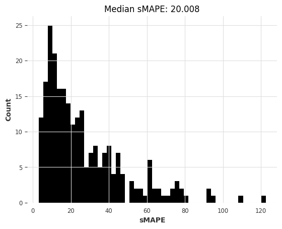
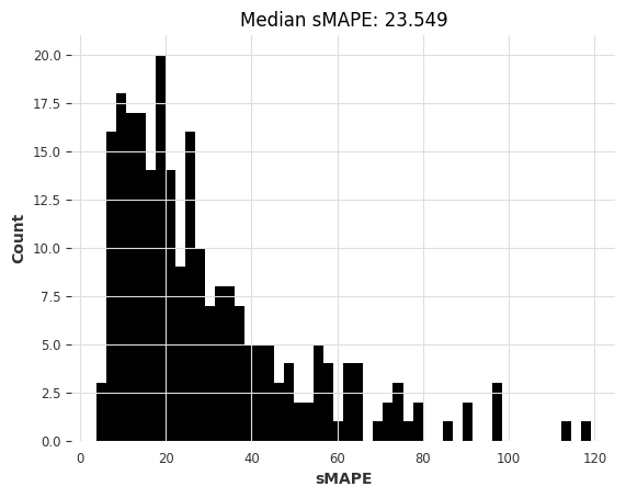
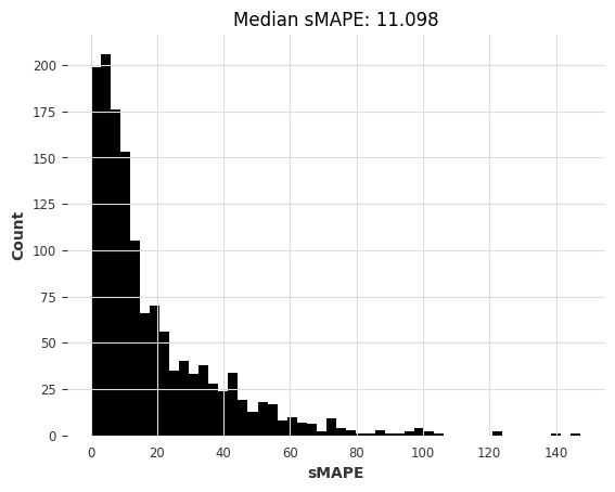
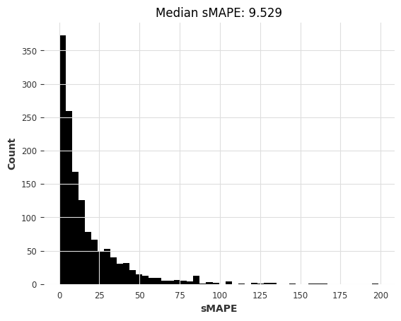
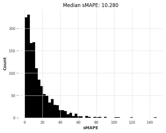
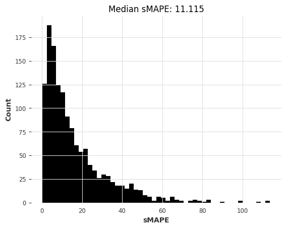
最后，我们定义一个便捷函数，用于告知我们一组预测序列的效果如何

def eval_forecasts(
    pred_series: list[TimeSeries], test_series: list[TimeSeries]
) -> list[float]:
    print("computing sMAPEs...")
    smapes = smape(test_series, pred_series)
    plt.figure()
    plt.hist(smapes, bins=50)
    plt.ylabel("Count")
    plt.xlabel("sMAPE")
    plt.title(f"Median sMAPE: {np.median(smapes):.3f}")
    plt.show()
    plt.close()
    return smapes

第 1 部分：在 air 数据集上使用局部模型

检查数据

air 数据集包含从 2000 年到 2019 年按承运商（或航空公司）划分的进出美国的航空乘客数量。

首先，我们可以通过调用上面定义的 load_air() 函数来加载训练和测试序列。

air_train, air_test = load_air()

IndexError: The type of your index was not matched.

splitting train/test...

IndexError: The type of your index was not matched.
IndexError: The type of your index was not matched.
IndexError: The type of your index was not matched.
IndexError: The type of your index was not matched.
IndexError: The type of your index was not matched.
IndexError: The type of your index was not matched.
IndexError: The type of your index was not matched.
IndexError: The type of your index was not matched.
IndexError: The type of your index was not matched.
IndexError: The type of your index was not matched.
IndexError: The type of your index was not matched.
IndexError: The type of your index was not matched.
IndexError: The type of your index was not matched.

scaling series...
done. There are 245 series, with average training length 154.06938775510204

首先可视化几个序列以了解其外观是个不错的主意。我们可以通过调用 series.plot() 来绘制序列。

figure, ax = plt.subplots(3, 2, figsize=(10, 10), dpi=100)

for i, idx in enumerate([1, 20, 50, 100, 150, 200]):
    axis = ax[i % 3, i % 2]
    air_train[idx].plot(ax=axis)
    axis.legend(air_train[idx].components)
    axis.set_title("")
plt.tight_layout()

我们可以看到大多数序列看起来差异很大，甚至有不同的时间轴！例如，有些序列始于 2001 年 1 月，而另一些则始于 2010 年 4 月。

让我们看看最短的可用训练序列是什么

min([len(s) for s in air_train])

36

一个用于评估模型的有用函数

下面，我们编写一个小型函数，以便快速尝试和比较不同的局部模型，从而使我们的工作更轻松。我们遍历每个序列，拟合模型，然后在测试数据集上进行评估。

⚠️ tqdm 是可选的，仅用于帮助显示训练进度（正如您将看到的，训练 300 多个时间序列可能需要一些时间）

def eval_local_model(
    train_series: list[TimeSeries], test_series: list[TimeSeries], model_cls, **kwargs
) -> tuple[list[float], float]:
    preds = []
    start_time = time.time()
    for series in tqdm(train_series):
        model = model_cls(**kwargs)
        model.fit(series)
        pred = model.predict(n=HORIZON)
        preds.append(pred)
    elapsed_time = time.time() - start_time

    smapes = eval_forecasts(preds, test_series)
    return smapes, elapsed_time

构建和评估模型

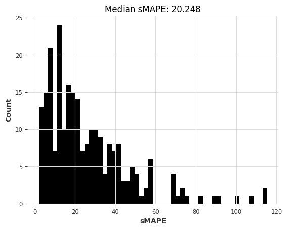
现在我们可以在此数据集上尝试第一个预测模型。第一步通常是查看一个（非常）朴素的模型，它盲目重复训练序列的最后一个值，看看其表现如何。这可以在 Darts 中使用 NaiveSeasonal 模型实现

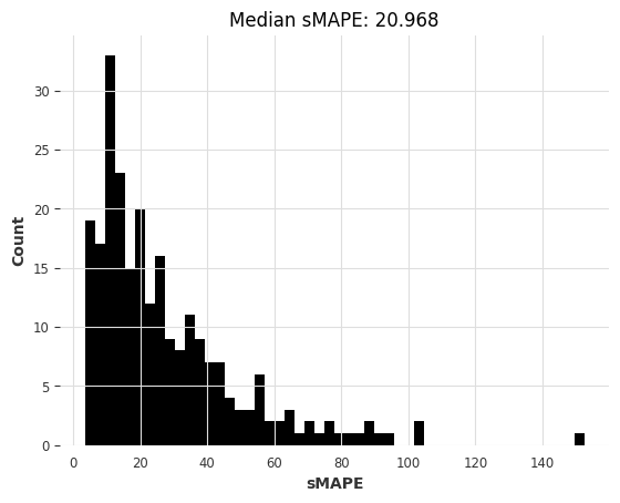
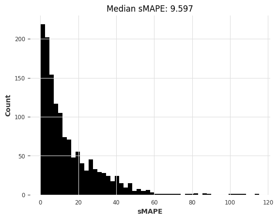
naive1_smapes, naive1_time = eval_local_model(air_train, air_test, NaiveSeasonal, K=1)

computing sMAPEs...

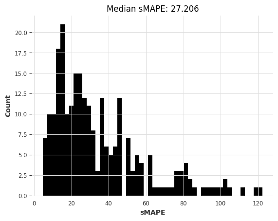
因此，最朴素的模型给出的中位数 sMAPE 约为 27.2。

我们能否使用一个“不那么朴素”的模型，利用大多数月度序列具有季节性为 12 的事实，从而做得更好？

naive12_smapes, naive12_time = eval_local_model(
    air_train, air_test, NaiveSeasonal, K=12
)

computing sMAPEs...

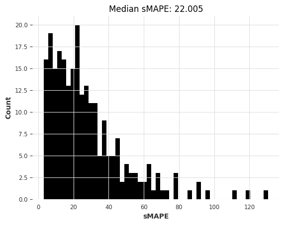
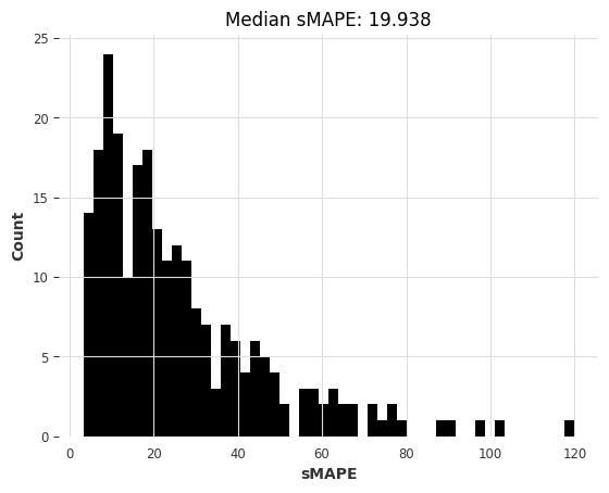
这更好。让我们尝试 ExponentialSmoothing（默认情况下，对于月度序列，它将使用季节性为 12）

ets_smapes, ets_time = eval_local_model(air_train, air_test, ExponentialSmoothing)

computing sMAPEs...

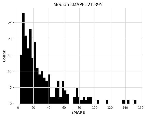
中位数略好于朴素季节性模型。我们可以快速尝试的另一个模型是赢得了 M3 竞赛的 Theta 方法

theta_smapes, theta_time = eval_local_model(air_train, air_test, Theta, theta=1.5)

computing sMAPEs...

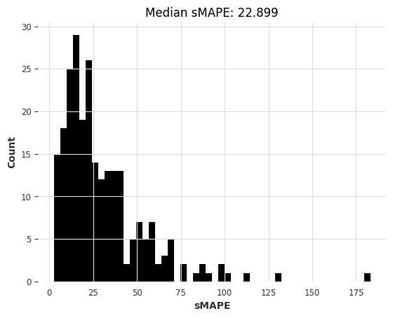
ARIMA 呢？

warnings.filterwarnings("ignore")  # ARIMA generates lots of warnings
arima_smapes, arima_time = eval_local_model(air_train, air_test, ARIMA, p=12, d=1, q=1)

computing sMAPEs...

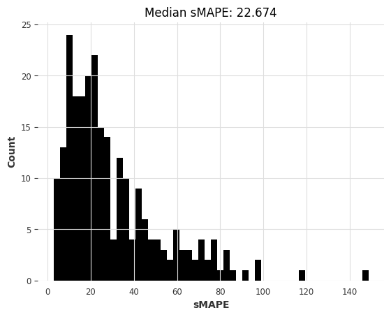
或者卡尔曼滤波？（在 Darts 中，拟合卡尔曼滤波器使用 N4SID 系统辨识算法）

kf_smapes, kf_time = eval_local_model(air_train, air_test, KalmanForecaster, dim_x=12)

computing sMAPEs...

比较模型

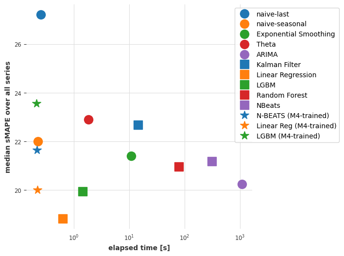
下面，我们定义一个函数，该函数对于可视化模型在中位数 sMAPE 以及获取预测所需时间方面的相互比较非常有用。

def plot_models(method_to_elapsed_times, method_to_smapes):
    shapes = ["o", "s", "*"]
    colors = ["tab:blue", "tab:orange", "tab:green", "tab:red", "tab:purple"]
    styles = list(product(shapes, colors))

    plt.figure(figsize=(6, 6), dpi=100)
    for i, method in enumerate(method_to_elapsed_times.keys()):
        t = method_to_elapsed_times[method]
        s = styles[i]
        plt.semilogx(
            [t],
            [np.median(method_to_smapes[method])],
            s[0],
            color=s[1],
            label=method,
            markersize=13,
        )
    plt.xlabel("elapsed time [s]")
    plt.ylabel("median sMAPE over all series")
    plt.legend(bbox_to_anchor=(1.4, 1.0), frameon=True)

smapes = {
    "naive-last": naive1_smapes,
    "naive-seasonal": naive12_smapes,
    "Exponential Smoothing": ets_smapes,
    "Theta": theta_smapes,
    "ARIMA": arima_smapes,
    "Kalman Filter": kf_smapes,
}

elapsed_times = {
    "naive-last": naive1_time,
    "naive-seasonal": naive12_time,
    "Exponential Smoothing": ets_time,
    "Theta": theta_time,
    "ARIMA": arima_time,
    "Kalman Filter": kf_time,
}

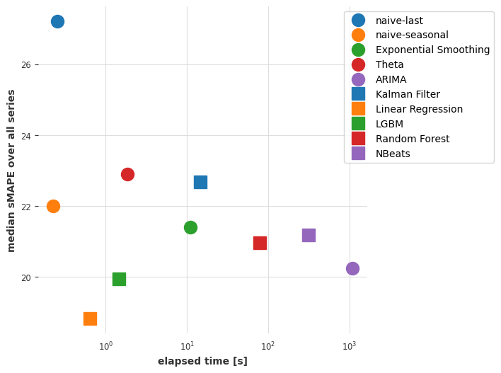
plot_models(elapsed_times, smapes)

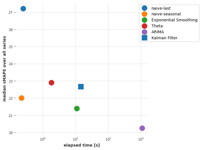
目前的结论

ARIMA 提供了最好的结果，但它也是（迄今为止）最耗时的模型。指数平滑模型提供了一个有趣的权衡，预测准确性好，计算成本较低。我们能否通过考虑全局模型——即仅一次性在所有时间序列上联合训练的模型——来找到更好的折衷方案？

第 2 部分：在 air 数据集上使用全局模型

在本节中，我们将使用“全局模型”——即一次性拟合多个序列的模型。Darts 主要有两种全局模型

• RegressionModels，它们是围绕类似 sklearn 的回归模型的封装器（第 2.1 部分）。

• 基于 PyTorch 的模型，提供各种深度学习模型（第 2.2 部分）。

这两种模型都可以通过将数据“表格化”在多个序列上进行训练——即从所有训练序列中提取许多（输入、输出）子切片，并以监督方式训练机器学习模型，以根据输入预测输出。

我们首先定义一个函数 eval_global_model()，它的工作方式类似于 eval_local_model()，但用于全局模型。

def eval_global_model(
    train_series: list[TimeSeries], test_series: list[TimeSeries], model_cls, **kwargs
) -> tuple[list[float], float]:
    start_time = time.time()

    model = model_cls(**kwargs)
    model.fit(train_series)
    preds = model.predict(n=HORIZON, series=train_series)

    elapsed_time = time.time() - start_time

    smapes = eval_forecasts(preds, test_series)
    return smapes, elapsed_time

第 2.1 部分：使用 Darts RegressionModel。

Darts 中的 RegressionModel 是预测模型，可以封装任何“scikit-learn 兼容”的回归模型来获取预测。与深度学习相比，它们是很好的“首选”全局模型，因为它们通常没有太多超参数，训练速度也更快。此外，Darts 还提供了一些“预打包”的回归模型，例如 LinearRegressionModel 和 LightGBMModel。

现在我们将使用我们的函数 eval_global_models()。在以下单元格中，我们将尝试使用一些回归模型，例如

• LinearRegressionModel

• LightGBMModel

• RegressionModel(some_sklearn_model)

您可以参考API 文档了解如何使用它们。

重要参数是 lags 和 output_chunk_length。它们分别决定模型使用的回溯窗口和“前瞻”窗口的长度，对应于用于训练的输入/输出子切片的长度。例如，lags=24 和 output_chunk_length=12 意味着模型将使用过去 24 个滞后项来预测未来 12 个滞后项。在我们的例子中，由于最短的训练序列长度为 36，我们必须满足 lags + output_chunk_length <= 36。（注意，lags 也可以是整数列表，表示模型需要使用的单个滞后项，而不是窗口长度）。

lr_smapes, lr_time = eval_global_model(
    air_train, air_test, LinearRegressionModel, lags=30, output_chunk_length=1
)

computing sMAPEs...

lgbm_smapes, lgbm_time = eval_global_model(
    air_train, air_test, LightGBMModel, lags=30, output_chunk_length=1, objective="mape"
)

[LightGBM] [Warning] Some label values are < 1 in absolute value. MAPE is unstable with such values, so LightGBM rounds them to 1.0 when calculating MAPE.
[LightGBM] [Info] Auto-choosing col-wise multi-threading, the overhead of testing was 0.003476 seconds.
You can set `force_col_wise=true` to remove the overhead.
[LightGBM] [Info] Total Bins 7649
[LightGBM] [Info] Number of data points in the train set: 30397, number of used features: 30
[LightGBM] [Info] Start training from score 0.481005
computing sMAPEs...

rf_smapes, rf_time = eval_global_model(
    air_train, air_test, RandomForest, lags=30, output_chunk_length=1
)

computing sMAPEs...

第 2.2 部分：使用深度学习

下面，我们将在 air 数据集上训练一个 N-BEATS 模型。同样，您可以参考API 文档了解超参数的文档。以下超参数应该是一个不错的起点，如果您使用（稍慢的）Colab GPU，训练大约需要一两分钟。

训练期间，您可以查看N-BEATS 论文。

### Possible N-BEATS hyper-parameters

# Slicing hyper-params:
IN_LEN = 30
OUT_LEN = 4

# Architecture hyper-params:
NUM_STACKS = 20
NUM_BLOCKS = 1
NUM_LAYERS = 2
LAYER_WIDTH = 136
COEFFS_DIM = 11

# Training settings:
LR = 1e-3
BATCH_SIZE = 1024
MAX_SAMPLES_PER_TS = 10
NUM_EPOCHS = 10

现在我们使用 N-BEATS 模型进行构建、训练和预测

# reproducibility
np.random.seed(42)
torch.manual_seed(42)

start_time = time.time()

nbeats_model_air = NBEATSModel(
    input_chunk_length=IN_LEN,
    output_chunk_length=OUT_LEN,
    num_stacks=NUM_STACKS,
    num_blocks=NUM_BLOCKS,
    num_layers=NUM_LAYERS,
    layer_widths=LAYER_WIDTH,
    expansion_coefficient_dim=COEFFS_DIM,
    loss_fn=SmapeLoss(),
    batch_size=BATCH_SIZE,
    optimizer_kwargs={"lr": LR},
    pl_trainer_kwargs={
        "enable_progress_bar": True,
        # change this one to "gpu" if your notebook does run in a GPU environment:
        "accelerator": "cpu",
    },
)

nbeats_model_air.fit(air_train, dataloader_kwargs={"num_workers": 4}, epochs=NUM_EPOCHS)

# get predictions
nb_preds = nbeats_model_air.predict(series=air_train, n=HORIZON)
nbeats_elapsed_time = time.time() - start_time

nbeats_smapes = eval_forecasts(nb_preds, air_test)

GPU available: True (mps), used: False
TPU available: False, using: 0 TPU cores
IPU available: False, using: 0 IPUs
HPU available: False, using: 0 HPUs

  | Name          | Type             | Params
---------------------------------------------------
0 | criterion     | SmapeLoss        | 0
1 | train_metrics | MetricCollection | 0
2 | val_metrics   | MetricCollection | 0
3 | stacks        | ModuleList       | 525 K
---------------------------------------------------
523 K     Trainable params
1.9 K     Non-trainable params
525 K     Total params
2.102     Total estimated model params size (MB)

`Trainer.fit` stopped: `max_epochs=10` reached.
GPU available: True (mps), used: False
TPU available: False, using: 0 TPU cores
IPU available: False, using: 0 IPUs
HPU available: False, using: 0 HPUs

computing sMAPEs...

现在我们再看看我们的误差-时间图

smapes_2 = {
    **smapes,
    **{
        "Linear Regression": lr_smapes,
        "LGBM": lgbm_smapes,
        "Random Forest": rf_smapes,
        "NBeats": nbeats_smapes,
    },
}

elapsed_times_2 = {
    **elapsed_times,
    **{
        "Linear Regression": lr_time,
        "LGBM": lgbm_time,
        "Random Forest": rf_time,
        "NBeats": nbeats_elapsed_time,
    },
}

plot_models(elapsed_times_2, smapes_2)

目前的结论

因此，看来联合训练所有序列的线性回归模型在准确性和速度之间提供了最佳权衡。线性回归通常是一个不错的选择！

我们的深度学习模型 N-BEATS 表现不佳。请注意，我们没有明确地为此问题调整它，这样做可能会产生更准确的结果。然而，与其花时间调整它，在下一部分中，我们将看看它是否可以通过在完全不同的数据集上进行训练来表现得更好。

第 3 部分：在 m4 数据集上训练 N-BEATS 模型并用其预测 air 数据集

深度学习模型在大型数据集上训练时通常表现更好。让我们尝试加载 M4 数据集中的全部 48,000 个月度时间序列，并在这个更大的数据集上再次训练我们的模型。

m4_train, m4_test = load_m4()

There are 47087 monthly series in the M3 dataset
scaling...
done. There are 47087 series, with average training length 201.25202285131778

我们可以从与之前相同的超参数开始。

M4 数据集中有 48,000 个训练序列，平均长度约为 200 个时间步长，最终我们将得到约 10M 个训练样本。如此多的训练样本会导致每个 epoch 耗时过长。因此，在此处，我们将限制每个序列使用的训练样本数量。这通过调用 fit() 并设置参数 max_samples_per_ts 来实现。我们添加一个新的超参数 MAX_SAMPLES_PER_TS 来表示这个限制。

由于 M4 训练序列都稍微长一些，我们也可以使用稍微长一些的 input_chunk_length。

# Slicing hyper-params:
IN_LEN = 36
OUT_LEN = 4

# Architecture hyper-params:
NUM_STACKS = 20
NUM_BLOCKS = 1
NUM_LAYERS = 2
LAYER_WIDTH = 136
COEFFS_DIM = 11

# Training settings:
LR = 1e-3
BATCH_SIZE = 1024
MAX_SAMPLES_PER_TS = (
    10  # <-- new parameter, limiting the number of training samples per series
)
NUM_EPOCHS = 5

# reproducibility
np.random.seed(42)
torch.manual_seed(42)

nbeats_model_m4 = NBEATSModel(
    input_chunk_length=IN_LEN,
    output_chunk_length=OUT_LEN,
    batch_size=BATCH_SIZE,
    num_stacks=NUM_STACKS,
    num_blocks=NUM_BLOCKS,
    num_layers=NUM_LAYERS,
    layer_widths=LAYER_WIDTH,
    expansion_coefficient_dim=COEFFS_DIM,
    loss_fn=SmapeLoss(),
    optimizer_kwargs={"lr": LR},
    pl_trainer_kwargs={
        "enable_progress_bar": True,
        # change this one to "gpu" if your notebook does run in a GPU environment:
        "accelerator": "cpu",
    },
)

# Train
nbeats_model_m4.fit(
    m4_train,
    dataloader_kwargs={"num_workers": 4},
    epochs=NUM_EPOCHS,
    max_samples_per_ts=MAX_SAMPLES_PER_TS,
)

GPU available: True (mps), used: False
TPU available: False, using: 0 TPU cores
IPU available: False, using: 0 IPUs
HPU available: False, using: 0 HPUs

  | Name          | Type             | Params
---------------------------------------------------
0 | criterion     | SmapeLoss        | 0
1 | train_metrics | MetricCollection | 0
2 | val_metrics   | MetricCollection | 0
3 | stacks        | ModuleList       | 543 K
---------------------------------------------------
541 K     Trainable params
1.9 K     Non-trainable params
543 K     Total params
2.173     Total estimated model params size (MB)

`Trainer.fit` stopped: `max_epochs=5` reached.

NBEATSModel(generic_architecture=True, num_stacks=20, num_blocks=1, num_layers=2, layer_widths=136, expansion_coefficient_dim=11, trend_polynomial_degree=2, dropout=0.0, activation=ReLU, input_chunk_length=36, output_chunk_length=4, batch_size=1024, loss_fn=SmapeLoss(), optimizer_kwargs={'lr': 0.001}, pl_trainer_kwargs={'enable_progress_bar': True, 'accelerator': 'cpu'})

现在我们可以使用在 M4 数据集上训练的模型来获取航空乘客序列的预测结果。由于我们在这里以“元学习”（或迁移学习）的方式使用模型，我们将只计时推理部分。

start_time = time.time()
preds = nbeats_model_m4.predict(series=air_train, n=HORIZON)  # get forecasts
nbeats_m4_elapsed_time = time.time() - start_time

nbeats_m4_smapes = eval_forecasts(preds, air_test)

GPU available: True (mps), used: False
TPU available: False, using: 0 TPU cores
IPU available: False, using: 0 IPUs
HPU available: False, using: 0 HPUs

computing sMAPEs...

smapes_3 = {**smapes_2, **{"N-BEATS (M4-trained)": nbeats_m4_smapes}}

elapsed_times_3 = {
    **elapsed_times_2,
    **{"N-BEATS (M4-trained)": nbeats_m4_elapsed_time},
}

plot_models(elapsed_times_3, smapes_3)

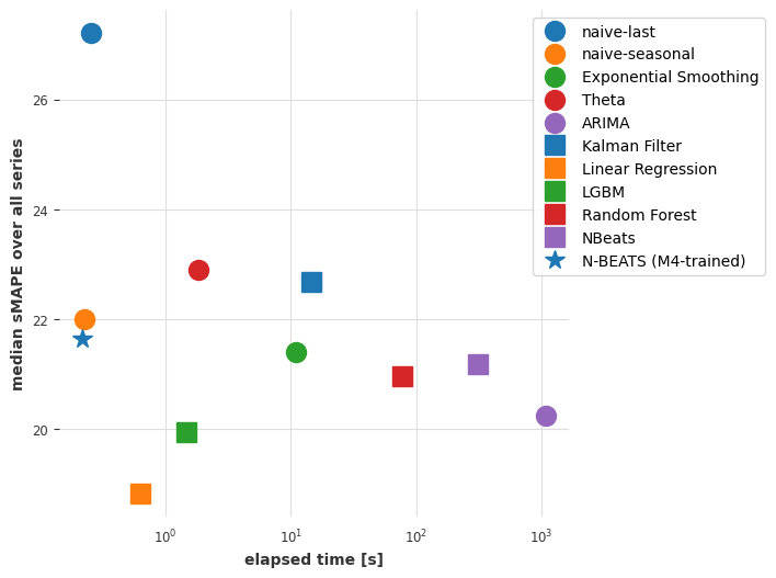
目前的结论

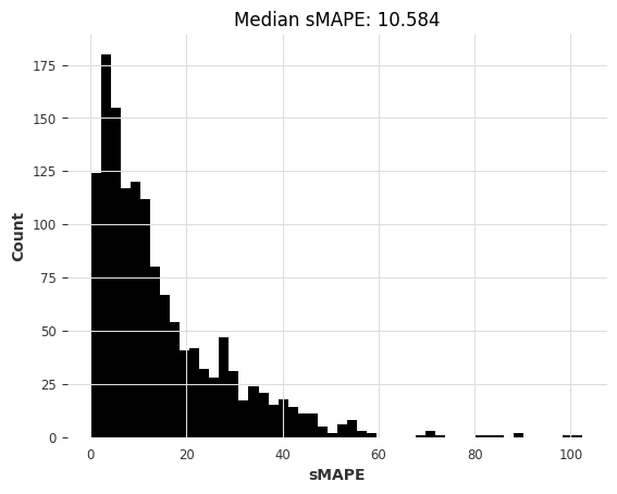
虽然在准确性方面它不是绝对最好的，但我们在 m4 上训练的 N-BEATS 模型达到了具有竞争力的准确性。这相当引人注目，因为该模型从未在我们要求它预测的任何 air 序列上进行过训练！使用 N-BEATS 进行预测的步骤比 ARIMA 所需的拟合-预测步骤快 1000 多倍，也比线性回归快。

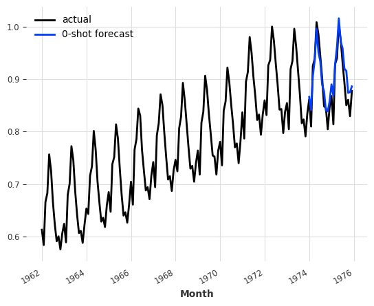
仅仅为了好玩，我们也可以手动检查这个模型在另一个序列上的表现——例如，darts.datasets 中提供的月度牛奶产量序列

from darts.datasets import MonthlyMilkDataset

series = MonthlyMilkDataset().load().astype(np.float32)
train, val = series[:-24], series[-24:]

scaler = Scaler(scaler=MaxAbsScaler())
train = scaler.fit_transform(train)
val = scaler.transform(val)
series = scaler.transform(series)
pred = nbeats_model_m4.predict(series=train, n=24)

series.plot(label="actual")
pred.plot(label="0-shot forecast")

GPU available: True (mps), used: False
TPU available: False, using: 0 TPU cores
IPU available: False, using: 0 IPUs
HPU available: False, using: 0 HPUs

<Axes: xlabel='Month'>

尝试在 m4 上训练其他全局模型并应用于航空乘客数据

现在我们尝试在 M4 数据集上训练其他全局模型，看看能否获得类似的结果。下面，我们将在完整的 m4 数据集上训练一些 RegressionModel。这可能会相当慢。为了加快训练速度，我们可以使用例如 random.choices(m4_train, k=5000) 代替 m4_train 来限制训练集的大小。我们也可以为 max_samples_per_ts 指定足够小的值来限制训练样本的数量。

random.seed(42)

lr_model_m4 = LinearRegressionModel(lags=30, output_chunk_length=1)
lr_model_m4.fit(m4_train)

tic = time.time()
preds = lr_model_m4.predict(n=HORIZON, series=air_train)
lr_time_transfer = time.time() - tic

lr_smapes_transfer = eval_forecasts(preds, air_test)

computing sMAPEs...

random.seed(42)

lgbm_model_m4 = LightGBMModel(lags=30, output_chunk_length=1, objective="mape")
lgbm_model_m4.fit(m4_train)

tic = time.time()
preds = lgbm_model_m4.predict(n=HORIZON, series=air_train)
lgbm_time_transfer = time.time() - tic

lgbm_smapes_transfer = eval_forecasts(preds, air_test)

[LightGBM] [Warning] Some label values are < 1 in absolute value. MAPE is unstable with such values, so LightGBM rounds them to 1.0 when calculating MAPE.
[LightGBM] [Info] Auto-choosing row-wise multi-threading, the overhead of testing was 0.097573 seconds.
You can set `force_row_wise=true` to remove the overhead.
And if memory is not enough, you can set `force_col_wise=true`.
[LightGBM] [Info] Total Bins 7650
[LightGBM] [Info] Number of data points in the train set: 8063744, number of used features: 30
[LightGBM] [Info] Start training from score 0.722222
computing sMAPEs...

最后，让我们也绘制这些新结果

smapes_4 = {
    **smapes_3,
    **{
        "Linear Reg (M4-trained)": lr_smapes_transfer,
        "LGBM (M4-trained)": lgbm_smapes_transfer,
    },
}

elapsed_times_4 = {
    **elapsed_times_3,
    **{
        "Linear Reg (M4-trained)": lr_time_transfer,
        "LGBM (M4-trained)": lgbm_time_transfer,
    },
}

plot_models(elapsed_times_4, smapes_4)

第 4 部分和回顾：在 M3 数据集上使用相同的模型

好的，现在，我们在航空乘客数据集上是否只是运气好？让我们通过在新的数据集上重复整个过程来看看 :) 您会发现这实际上只需要很少的代码。作为新的数据集，我们将使用 m3，它包含来自 M3 竞赛的约 1,400 个月度序列。

m3_train, m3_test = load_m3()

building M3 TimeSeries...

There are 1399 monthly series in the M3 dataset
splitting train/test...
scaling...
done. There are 1399 series, with average training length 100.30092923516797

naive1_smapes_m3, naive1_time_m3 = eval_local_model(
    m3_train, m3_test, NaiveSeasonal, K=1
)

computing sMAPEs...

naive12_smapes_m3, naive12_time_m3 = eval_local_model(
    m3_train, m3_test, NaiveSeasonal, K=12
)

computing sMAPEs...

ets_smapes_m3, ets_time_m3 = eval_local_model(m3_train, m3_test, ExponentialSmoothing)

computing sMAPEs...

theta_smapes_m3, theta_time_m3 = eval_local_model(m3_train, m3_test, Theta)

computing sMAPEs...

warnings.filterwarnings("ignore")  # ARIMA generates lots of warnings

# Note: using q=1 here generates errors for some series, so we use q=0
arima_smapes_m3, arima_time_m3 = eval_local_model(
    m3_train, m3_test, ARIMA, p=12, d=1, q=0
)

computing sMAPEs...

kf_smapes_m3, kf_time_m3 = eval_local_model(
    m3_train, m3_test, KalmanForecaster, dim_x=12
)

computing sMAPEs...

lr_smapes_m3, lr_time_m3 = eval_global_model(
    m3_train, m3_test, LinearRegressionModel, lags=30, output_chunk_length=1
)

computing sMAPEs...

lgbm_smapes_m3, lgbm_time_m3 = eval_global_model(
    m3_train, m3_test, LightGBMModel, lags=35, output_chunk_length=1, objective="mape"
)

[LightGBM] [Warning] Some label values are < 1 in absolute value. MAPE is unstable with such values, so LightGBM rounds them to 1.0 when calculating MAPE.
[LightGBM] [Info] Auto-choosing col-wise multi-threading, the overhead of testing was 0.004819 seconds.
You can set `force_col_wise=true` to remove the overhead.
[LightGBM] [Info] Total Bins 8925
[LightGBM] [Info] Number of data points in the train set: 91356, number of used features: 35
[LightGBM] [Info] Start training from score 0.771293
computing sMAPEs...

# Get forecasts with our pre-trained N-BEATS

start_time = time.time()
preds = nbeats_model_m4.predict(series=m3_train, n=HORIZON)  # get forecasts
nbeats_m4_elapsed_time_m3 = time.time() - start_time

nbeats_m4_smapes_m3 = eval_forecasts(preds, m3_test)

GPU available: True (mps), used: False
TPU available: False, using: 0 TPU cores
IPU available: False, using: 0 IPUs
HPU available: False, using: 0 HPUs

computing sMAPEs...

# Get forecasts with our pre-trained linear regression model

start_time = time.time()
preds = lr_model_m4.predict(series=m3_train, n=HORIZON)  # get forecasts
lr_m4_elapsed_time_m3 = time.time() - start_time

lr_m4_smapes_m3 = eval_forecasts(preds, m3_test)

computing sMAPEs...

# Get forecasts with our pre-trained LightGBM model

start_time = time.time()
preds = lgbm_model_m4.predict(series=m3_train, n=HORIZON)  # get forecasts
lgbm_m4_elapsed_time_m3 = time.time() - start_time

lgbm_m4_smapes_m3 = eval_forecasts(preds, m3_test)

computing sMAPEs...

smapes_m3 = {
    "naive-last": naive1_smapes_m3,
    "naive-seasonal": naive12_smapes_m3,
    "Exponential Smoothing": ets_smapes_m3,
    "ARIMA": arima_smapes_m3,
    "Theta": theta_smapes_m3,
    "Kalman filter": kf_smapes_m3,
    "Linear Regression": lr_smapes_m3,
    "LGBM": lgbm_smapes_m3,
    "N-BEATS (M4-trained)": nbeats_m4_smapes_m3,
    "Linear Reg (M4-trained)": lr_m4_smapes_m3,
    "LGBM (M4-trained)": lgbm_m4_smapes_m3,
}

times_m3 = {
    "naive-last": naive1_time_m3,
    "naive-seasonal": naive12_time_m3,
    "Exponential Smoothing": ets_time_m3,
    "ARIMA": arima_time_m3,
    "Theta": theta_time_m3,
    "Kalman filter": kf_time_m3,
    "Linear Regression": lr_time_m3,
    "LGBM": lgbm_time_m3,
    "N-BEATS (M4-trained)": nbeats_m4_elapsed_time_m3,
    "Linear Reg (M4-trained)": lr_m4_elapsed_time_m3,
    "LGBM (M4-trained)": lgbm_m4_elapsed_time_m3,
}

plot_models(times_m3, smapes_m3)

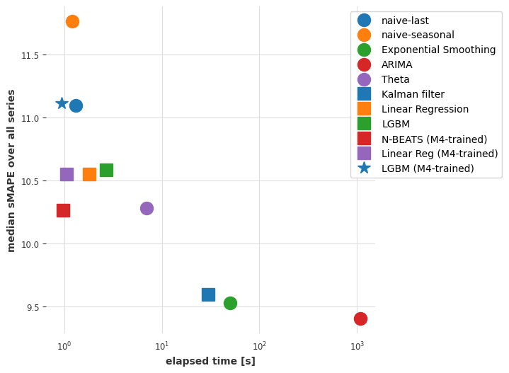
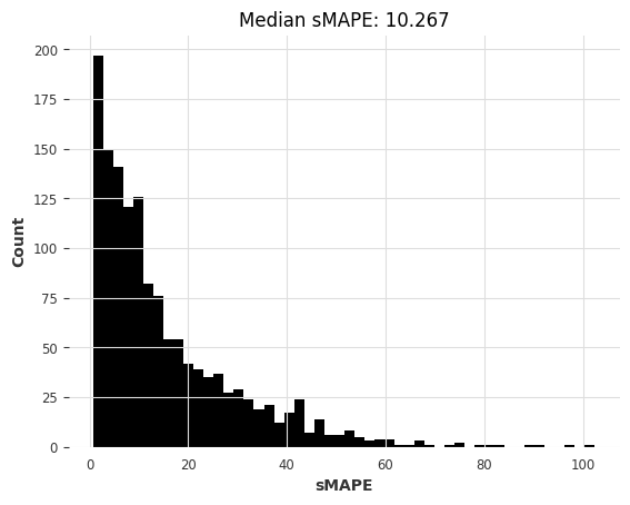
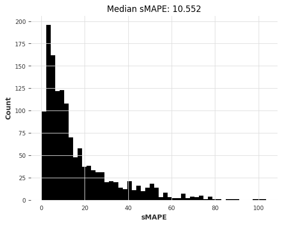
在这里，预训练的 N-BEATS 模型也获得了合理的准确性，尽管不如最准确的模型。另请注意，指数平滑和卡尔曼滤波现在表现得比我们在航空乘客序列上使用时要好得多。ARIMA 表现最好，但比 N-BEATS 慢约 1000 倍，N-BEATS 不需要任何训练，生成其预测结果每个时间序列大约需要 15 毫秒。请记住，这个 N-BEATS 模型从未在我们要求它预测的任何序列上进行过训练。

结论

迁移学习和元学习无疑是一个有趣的现象，目前在时间序列预测中仍未得到充分探索。它何时成功？何时失败？微调是否有帮助？何时应该使用？这些问题中的许多仍有待探索，但我们希望通过 Darts 模型已经表明，这样做是相当容易的。

那么，哪种方法最适合您的情况？一如既往，这取决于具体情况。如果您主要处理具有足够历史的孤立序列，经典方法如 ARIMA 将大有裨益。即使在更大的数据集上，如果计算能力不是太大问题，它们也可以提供有趣的开箱即用选项。另一方面，如果您处理大量序列或更高维度的序列，机器学习方法和全局模型通常是首选。它们可以捕获不同时间序列之间的广泛模式，并且通常运行速度更快。不要低估基于线性回归的模型！如果您有理由相信需要捕获更复杂的模式，或者如果推理速度对您确实重要，请尝试深度学习方法。N-BEATS 在元学习中已经证明了其价值 [1]，但这可能也适用于其他模型。

[1] Oreshkin et al., “Meta-learning framework with applications to zero-shot time-series forecasting”, 2020, https://arxiv.org/abs/2002.02887

上一页

静态协变量

下一页

分层协调 - 澳大利亚旅游数据集示例