时间序列混合器 (TSMixer)
本笔记本演示了如何使用 Darts 的 TSMixerModel 并将其与 TiDEModel 进行基准测试。
TSMixer (时间序列混合器) 是一种用于时间序列预测的全 MLP 架构。
它通过集成历史时间序列数据、未来已知输入和静态上下文信息来实现。该架构结合使用了条件特征混合和混合器层来处理和组合这些不同类型的数据,以实现有效的预测。
翻译到 Darts 中,这个模型支持所有类型的协变量(过去、未来和/或静态)。
查看原始论文和模型描述 此处。
据作者称,该模型在多元预测任务上优于几个最先进的模型。
让我们看看它在 ETTh1 和 ETTh2 数据集上与 TiDEModel 相比表现如何。
[1]:
# fix python path if working locally
from utils import fix_pythonpath_if_working_locally

fix_pythonpath_if_working_locally()
%matplotlib inline
[2]:
%load_ext autoreload
%autoreload 2
%matplotlib inline
[3]:
import warnings

warnings.filterwarnings("ignore")
import logging

logging.disable(logging.CRITICAL)

import matplotlib.pyplot as plt
import numpy as np
import pandas as pd
import torch
from pytorch_lightning.callbacks.early_stopping import EarlyStopping

from darts import concatenate
from darts.dataprocessing.transformers.scaler import Scaler
from darts.datasets import ETTh1Dataset, ETTh2Dataset
from darts.metrics import mql
from darts.models import TiDEModel, TSMixerModel
from darts.utils.callbacks import TFMProgressBar
from darts.utils.likelihood_models.torch import QuantileRegression
数据加载与准备
我们考虑 ETTh1 和 ETTh2 数据集,其中包含电力变压器的小时级多元数据(负荷、油温等)。你可以在 此处 找到更多信息。
我们将向每个变压器时间序列添加静态信息,用于识别它是 ETTh1 变压器还是 ETTh2 变压器。TSMixer 和 TiDE 都可以利用这些信息。
[4]:
series = []
for idx, ds in enumerate([ETTh1Dataset, ETTh2Dataset]):
    trafo = ds().load().astype(np.float32)
    trafo = trafo.with_static_covariates(pd.DataFrame({"transformer_id": [idx]}))
    series.append(trafo)
series[0].to_dataframe()
[4]:
| 分量 | HUFL | HULL | MUFL | MULL | LUFL | LULL | OT |
|---|---|---|---|---|---|---|---|
| 日期 | |||||||
| 2016-07-01 00:00:00 | 5.827 | 2.009 | 1.599 | 0.462 | 4.203 | 1.340 | 30.531000 |
| 2016-07-01 01:00:00 | 5.693 | 2.076 | 1.492 | 0.426 | 4.142 | 1.371 | 27.787001 |
| 2016-07-01 02:00:00 | 5.157 | 1.741 | 1.279 | 0.355 | 3.777 | 1.218 | 27.787001 |
| 2016-07-01 03:00:00 | 5.090 | 1.942 | 1.279 | 0.391 | 3.807 | 1.279 | 25.044001 |
| 2016-07-01 04:00:00 | 5.358 | 1.942 | 1.492 | 0.462 | 3.868 | 1.279 | 21.948000 |
| ... | ... | ... | ... | ... | ... | ... | ... |
| 2018-06-26 15:00:00 | -1.674 | 3.550 | -5.615 | 2.132 | 3.472 | 1.523 | 10.904000 |
| 2018-06-26 16:00:00 | -5.492 | 4.287 | -9.132 | 2.274 | 3.533 | 1.675 | 11.044000 |
| 2018-06-26 17:00:00 | 2.813 | 3.818 | -0.817 | 2.097 | 3.716 | 1.523 | 10.271000 |
| 2018-06-26 18:00:00 | 9.243 | 3.818 | 5.472 | 2.097 | 3.655 | 1.432 | 9.778000 |
| 2018-06-26 19:00:00 | 10.114 | 3.550 | 6.183 | 1.564 | 3.716 | 1.462 | 9.567000 |
17420 行 × 7 列
在训练之前,我们将数据分割为训练集、验证集和测试集。模型将从训练集中学习,使用验证集来决定何时停止训练,最后在测试集上进行评估。
[5]:
train, val, test = [], [], []
for trafo in series:
    train_, temp = trafo.split_after(0.6)
    val_, test_ = temp.split_after(0.5)
    train.append(train_)
    val.append(val_)
    test.append(test_)
让我们看看对于每个变压器的第一个列“HUFL”的分割情况。
[6]:
show_col = "HUFL"
for idx, (train_, val_, test_) in enumerate(zip(train, val, test)):
    train_[show_col].plot(label=f"train_trafo_{idx}")
    val_[show_col].plot(label=f"val_trafo_{idx}")
    test_[show_col].plot(label=f"test_trafo_{idx}")
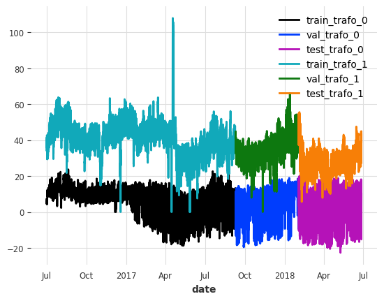
现在我们来缩放数据。为了避免从验证集和测试集中泄露信息,我们根据训练集的属性来缩放数据。
[7]:
scaler = Scaler()  # default uses sklearn's MinMaxScaler
train = scaler.fit_transform(train)
val = scaler.transform(val)
test = scaler.transform(test)
模型参数设置
模板代码很无聊,特别是在训练多个模型进行性能比较时。为了避免这种情况,我们使用一个通用配置,该配置可以用于任何 Darts 的 TorchForecastingModel。
关于这些参数的一些有趣之处
梯度裁剪: 通过为批量梯度设置上限,减轻反向传播过程中的梯度爆炸问题。
学习率: 模型的大部分学习发生在早期 epochs。随着训练的进行,降低学习率通常有助于微调模型。话虽如此,它也可能导致严重的过拟合。
早停: 为了避免过拟合,我们可以使用早停。它监视验证集上的一个指标,并在指标根据自定义条件不再改进时停止训练。
似然函数和损失函数: 你可以使用
likelihood使模型具有概率性,或使用loss_fn使其具有确定性。在本笔记本中,我们使用 QuantileRegression 训练概率模型。可逆实例归一化: 使用 可逆实例归一化,这在大多数情况下都能提高模型性能。
编码器: 我们可以对时间轴/日历信息进行编码,并使用
add_encoders将它们用作过去或未来协变量。在这里,我们将添加小时、星期和月份的循环编码作为未来协变量。
[8]:
def create_params(
    input_chunk_length: int,
    output_chunk_length: int,
    full_training=True,
):
    # early stopping: this setting stops training once the the validation
    # loss has not decreased by more than 1e-5 for 10 epochs
    early_stopper = EarlyStopping(
        monitor="val_loss",
        patience=10,
        min_delta=1e-5,
        mode="min",
    )

    # PyTorch Lightning Trainer arguments (you can add any custom callback)
    if full_training:
        limit_train_batches = None
        limit_val_batches = None
        max_epochs = 200
        batch_size = 256
    else:
        limit_train_batches = 20
        limit_val_batches = 10
        max_epochs = 40
        batch_size = 64

    # only show the training and prediction progress bars
    progress_bar = TFMProgressBar(
        enable_sanity_check_bar=False, enable_validation_bar=False
    )
    pl_trainer_kwargs = {
        "gradient_clip_val": 1,
        "max_epochs": max_epochs,
        "limit_train_batches": limit_train_batches,
        "limit_val_batches": limit_val_batches,
        "accelerator": "auto",
        "callbacks": [early_stopper, progress_bar],
    }

    # optimizer setup, uses Adam by default
    # optimizer_cls = torch.optim.Adam
    optimizer_kwargs = {
        "lr": 1e-4,
    }

    # learning rate scheduler
    lr_scheduler_cls = torch.optim.lr_scheduler.ExponentialLR
    lr_scheduler_kwargs = {"gamma": 0.999}

    # for probabilistic models, we use quantile regression, and set `loss_fn` to `None`
    likelihood = QuantileRegression()
    loss_fn = None

    return {
        "input_chunk_length": input_chunk_length,  # lookback window
        "output_chunk_length": output_chunk_length,  # forecast/lookahead window
        "use_reversible_instance_norm": True,
        "optimizer_kwargs": optimizer_kwargs,
        "pl_trainer_kwargs": pl_trainer_kwargs,
        "lr_scheduler_cls": lr_scheduler_cls,
        "lr_scheduler_kwargs": lr_scheduler_kwargs,
        "likelihood": likelihood,  # use a `likelihood` for probabilistic forecasts
        "loss_fn": loss_fn,  # use a `loss_fn` for determinsitic model
        "save_checkpoints": True,  # checkpoint to retrieve the best performing model state,
        "force_reset": True,
        "batch_size": batch_size,
        "random_state": 42,
        "add_encoders": {
            "cyclic": {
                "future": ["hour", "dayofweek", "month"]
            }  # add cyclic time axis encodings as future covariates
        },
    }
模型配置
让我们使用最后一周的小时数据作为回溯窗口(input_chunk_length),并训练一个概率模型直接预测未来 24 小时(output_chunk_length)。此外,我们告诉模型使用静态信息。为了简化笔记本,我们将设置 full_training=False。为了获得更好的性能,请将 full_training=True。
除此之外,我们使用我们的辅助函数来设置所有通用模型参数。
[9]:
input_chunk_length = 7 * 24
output_chunk_length = 24
use_static_covariates = True
full_training = False
[10]:
# create the models
model_tsm = TSMixerModel(
    **create_params(
        input_chunk_length,
        output_chunk_length,
        full_training=full_training,
    ),
    use_static_covariates=use_static_covariates,
    model_name="tsm",
)
model_tide = TiDEModel(
    **create_params(
        input_chunk_length,
        output_chunk_length,
        full_training=full_training,
    ),
    use_static_covariates=use_static_covariates,
    model_name="tide",
)
models = {
    "TSM": model_tsm,
    "TiDE": model_tide,
}
模型训练
现在让我们训练所有模型。使用早停时,保存检查点很重要。这使我们可以在超过最佳模型配置后继续,然后一旦训练完成,即可恢复最优权重。
[11]:
# train the models and load the model from its best state/checkpoint
for model_name, model in models.items():
    model.fit(
        series=train,
        val_series=val,
    )
    # load from checkpoint returns a new model object, we store it in the models dict
    models[model_name] = model.load_from_checkpoint(
        model_name=model.model_name, best=True
    )
回测概率模型
让我们配置预测。在此示例中,我们将
使用预训练模型在测试集上生成历史预测。每个预测覆盖 24 小时的时间范围,并且两个连续预测之间的时间间隔也是 24 小时。这将为我们提供每个变压器的 276 个多元预测来评估模型!
对于每个预测点生成500 个随机样本(因为我们训练了概率模型)
评估/回测一些分位数的概率历史预测,使用平均分位数损失(
mql())。
我们还将创建一些辅助函数,用于生成预测、计算回测和可视化预测。
[12]:
# configure the probabilistic prediction
num_samples = 500
forecast_horizon = output_chunk_length
# compute the Mean Quantile Loss over these quantiles
evaluate_quantiles = [0.05, 0.1, 0.2, 0.5, 0.8, 0.9, 0.95]
def historical_forecasts(model):
"""Generates probabilistic historical forecasts for each transformer
and returns the inverse transformed results.
Each forecast covers 24h (forecast_horizon). The time between two forecasts
(stride) is also 24 hours.
"""
hfc = model.historical_forecasts(
series=test,
forecast_horizon=forecast_horizon,
stride=forecast_horizon,
last_points_only=False,
retrain=False,
num_samples=num_samples,
verbose=True,
)
return scaler.inverse_transform(hfc)
def backtest(model, hfc, name):
"""Evaluates probabilistic historical forecasts using the Mean Quantile
Loss (MQL) over a set of quantiles."""
# add metric specific kwargs
metric_kwargs = [{"q": q} for q in evaluate_quantiles]
metrics = [mql for _ in range(len(evaluate_quantiles))]
bt = model.backtest(
series=series,
historical_forecasts=hfc,
last_points_only=False,
metric=metrics,
metric_kwargs=metric_kwargs,
verbose=True,
)
bt = pd.DataFrame(
bt,
columns=[f"q_{q}" for q in evaluate_quantiles],
index=[f"{trafo}_{name}" for trafo in ["ETTh1", "ETTh2"]],
)
return bt
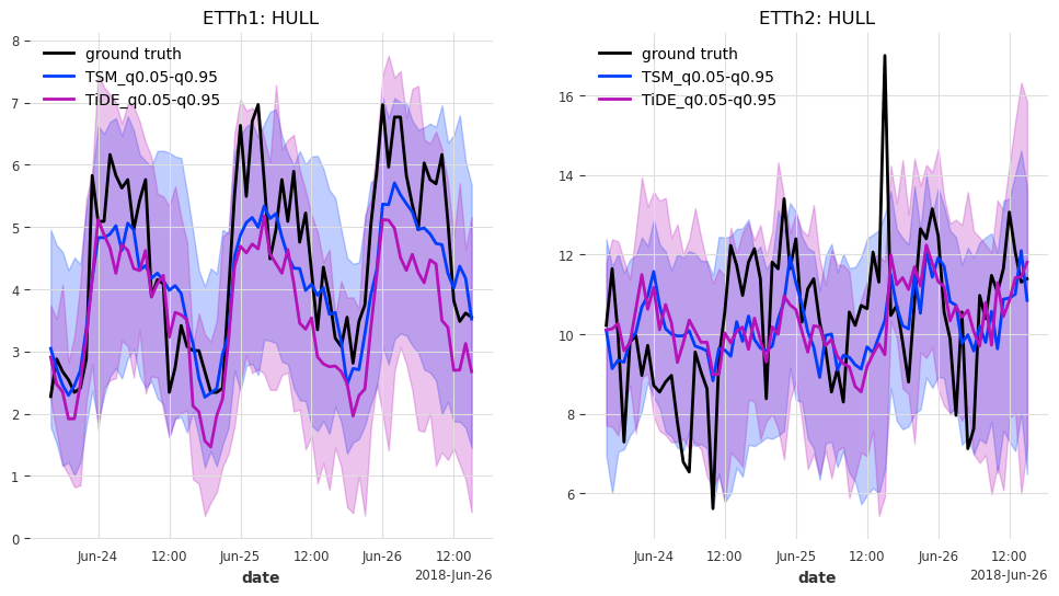
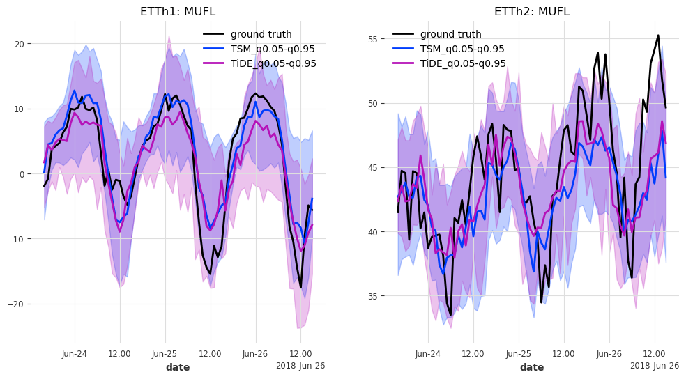
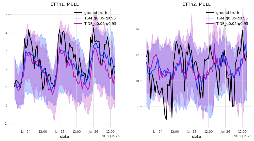
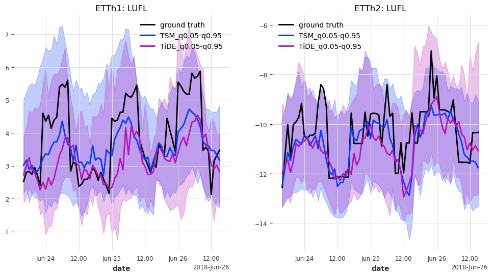
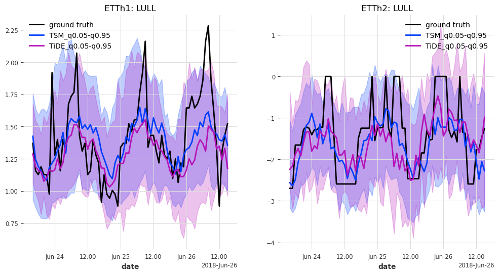
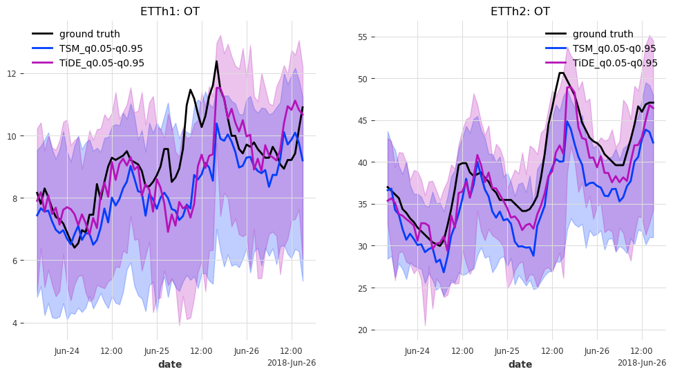
def generate_plots(n_days, hfcs):
"""Plot the probabilistic forecasts for each model, transformer and transformer
feature against the ground truth."""
# concatenate historical forecasts into contiguous time series
# (works because forecast_horizon=stride)
hfcs_plot = {}
for model_name, hfc_model in hfcs.items():
hfcs_plot[model_name] = [
concatenate(hfc_series[-n_days:], axis=0) for hfc_series in hfc_model
]
# remember start and end points for plotting the target series
hfc_ = hfcs_plot[model_name][0]
start, end = hfc_.start_time(), hfc_.end_time()
# for each target column...
for col in series[0].columns:
fig, axes = plt.subplots(ncols=2, figsize=(12, 6))
# ... and for each transformer...
for trafo_idx, trafo in enumerate(series):
trafo[col][start:end].plot(label="ground truth", ax=axes[trafo_idx])
# ... plot the historical forecasts for each model
for model_name, hfc in hfcs_plot.items():
hfc[trafo_idx][col].plot(
label=model_name + "_q0.05-q0.95", ax=axes[trafo_idx]
)
axes[trafo_idx].set_title(f"ETTh{trafo_idx + 1}: {col}")
plt.show()
好的,现在我们准备好评估模型了。
[13]:
bts = {}
hfcs = {}
for model_name, model in models.items():
    print(f"Model: {model_name}")
    print("Generating historical forecasts..")
    hfcs[model_name] = historical_forecasts(models[model_name])

    print("Evaluating historical forecasts..")
    bts[model_name] = backtest(models[model_name], hfcs[model_name], model_name)
Model: TSM
Generating historical forecasts..
Evaluating historical forecasts..
Model: TiDE
Generating historical forecasts..
Evaluating historical forecasts..
让我们看看它们的表现。
注意: 当设置
full_training=True时,这些结果可能会改善/改变。
[14]:
bt_df = pd.concat(bts.values(), axis=0).sort_index()
bt_df
[14]:
| q_0.05 | q_0.1 | q_0.2 | q_0.5 | q_0.8 | q_0.9 | q_0.95 | |
|---|---|---|---|---|---|---|---|
| ETTh1_TSM | 0.501772 | 0.769545 | 1.136141 | 1.568439 | 1.098847 | 0.721835 | 0.442062 |
| ETTh1_TiDE | 0.573716 | 0.885452 | 1.298672 | 1.671870 | 1.151501 | 0.727515 | 0.446724 |
| ETTh2_TSM | 0.659187 | 1.030655 | 1.508628 | 1.932923 | 1.317960 | 0.857147 | 0.524620 |
| ETTh2_TiDE | 0.627251 | 0.982114 | 1.450893 | 1.897117 | 1.323661 | 0.862239 | 0.528638 |
回测结果提供了对于每个变压器和模型的所有变压器特征的选定分位数的平均分位数损失。值越低越好。q_0.5 与中位数预测和地面真值之间的平均绝对误差 (MAE) 相同。
两个模型似乎都表现得相当好。所有分位数的平均表现如何?
[15]:
bt_df.mean(axis=1)
[15]:
ETTh1_TSM     0.891234
ETTh1_TiDE    0.965064
ETTh2_TSM     1.118732
ETTh2_TiDE    1.095988
dtype: float64
这里的结果也非常相似。TSMixer 在 ETTh1 上表现更好,而 TiDEModel 在 ETTh2 上表现更好。
最后但同样重要,让我们看看测试集中最后 n_days=3 天的预测结果。
注意:当
full_training=True时,预测区间预计会变窄。
[16]:
generate_plots(n_days=3, hfcs=hfcs)
结果
在本例中,TSMixer 和 TiDEModel 都表现得相当好。请记住,我们只对数据进行了部分训练,并且我们使用了默认模型参数,没有进行任何超参数调优。
以下是一些进一步提高性能的方法
设置
full_training=True执行超参数调优
添加更多协变量(我们只添加了日历信息的循环编码)
…
[ ]: