使用 `DataTransformer` 和 `Pipeline` 进行数据（预）处理¶

在本 notebook 中，我们将演示如何使用 darts 执行一些常见的预处理任务

`DataTransformer` 抽象¶

DataTransformer 旨在提供一种处理 TimeSeries 变换的统一方式

所有转换器都实现了 transform() 方法。该方法接受一个 TimeSeries 或一个 TimeSeries 序列作为输入，应用变换并将其作为新的 TimeSeries/TimeSeries 序列返回。
inverse_transform() 由存在逆变换函数的转换器实现。它的工作方式与 transform() 类似
fit() 允许转换器在调用 transform() 或 inverse_transform() 之前先从时间序列中提取一些信息

设置示例¶

[1]:

# fix python path if working locally
from utils import fix_pythonpath_if_working_locally

fix_pythonpath_if_working_locally()

%load_ext autoreload
%autoreload 2
%matplotlib inline

[2]:

import warnings

import matplotlib.pyplot as plt
import pandas as pd

from darts.dataprocessing import Pipeline
from darts.dataprocessing.transformers import (
    InvertibleMapper,
    Mapper,
    MissingValuesFiller,
    Scaler,
)
from darts.datasets import MonthlyMilkDataset, MonthlyMilkIncompleteDataset
from darts.metrics import mape
from darts.models import ExponentialSmoothing
from darts.utils.timeseries_generation import linear_timeseries

warnings.filterwarnings("ignore")
import logging

logging.disable(logging.CRITICAL)

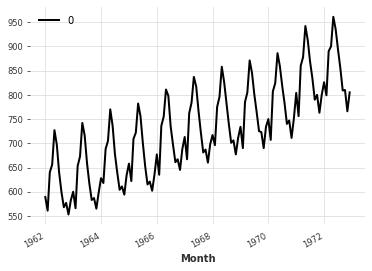
读取数据并创建时间序列¶

[3]:

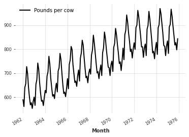
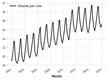
series = MonthlyMilkDataset().load()

print(series)
series.plot()

<TimeSeries (DataArray) (Month: 168, component: 1, sample: 1)>
array([[[589.]],

       [[561.]],

       [[640.]],

       [[656.]],

       [[727.]],

       [[697.]],

       [[640.]],

       [[599.]],

       [[568.]],

       [[577.]],

...

       [[892.]],

       [[903.]],

       [[966.]],

       [[937.]],

       [[896.]],

       [[858.]],

       [[817.]],

       [[827.]],

       [[797.]],

       [[843.]]])
Coordinates:
  * Month      (Month) datetime64[ns] 1962-01-01 1962-02-01 ... 1975-12-01
  * component  (component) object 'Pounds per cow'
Dimensions without coordinates: sample

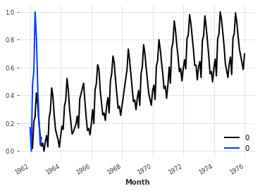
../_images/examples_02-data-processing_6_1.png

使用转换器：使用 `Scaler` 重缩放时间序列。¶

某些应用可能要求您的数据点介于 0 和 1 之间（例如，将时间序列馈送到基于神经网络的预测模型）。这很容易通过使用默认的 Scaler 实现，它是 sklearn.preprocessing.MinMaxScaler(feature_range=(0, 1)) 的封装。

[4]:

scaler = Scaler()
rescaled = scaler.fit_transform(series)
print(rescaled)

<TimeSeries (DataArray) (Month: 168, component: 1, sample: 1)>
array([[[0.08653846]],

       [[0.01923077]],

       [[0.20913462]],

       [[0.24759615]],

       [[0.41826923]],

       [[0.34615385]],

       [[0.20913462]],

       [[0.11057692]],

       [[0.03605769]],

       [[0.05769231]],

...

       [[0.81490385]],

       [[0.84134615]],

       [[0.99278846]],

       [[0.92307692]],

       [[0.82451923]],

       [[0.73317308]],

       [[0.63461538]],

       [[0.65865385]],

       [[0.58653846]],

       [[0.69711538]]])
Coordinates:
  * Month      (Month) datetime64[ns] 1962-01-01 1962-02-01 ... 1975-12-01
  * component  (component) <U1 '0'
Dimensions without coordinates: sample

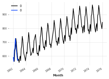
这种缩放也可以通过调用 inverse_transform() 轻松反转

[5]:

back = scaler.inverse_transform(rescaled)
print(back)

<TimeSeries (DataArray) (Month: 168, component: 1, sample: 1)>
array([[[589.]],

       [[561.]],

       [[640.]],

       [[656.]],

       [[727.]],

       [[697.]],

       [[640.]],

       [[599.]],

       [[568.]],

       [[577.]],

...

       [[892.]],

       [[903.]],

       [[966.]],

       [[937.]],

       [[896.]],

       [[858.]],

       [[817.]],

       [[827.]],

       [[797.]],

       [[843.]]])
Coordinates:
  * Month      (Month) datetime64[ns] 1962-01-01 1962-02-01 ... 1975-12-01
  * component  (component) <U1 '0'
Dimensions without coordinates: sample

请注意，Scaler 也允许在其构造函数中指定其他缩放器，只要它们在 TimeSeries 上实现了 fit()、transform() 和 inverse_transform() 方法（通常是 scikit-learn 中的缩放器）

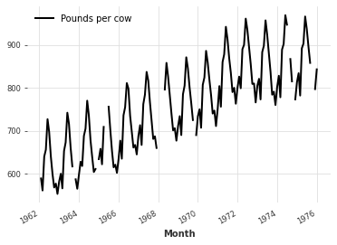
另一个例子：`MissingValuesFiller`¶

让我们看看如何处理数据集中的缺失值。

[6]:

incomplete_series = MonthlyMilkIncompleteDataset().load()
incomplete_series.plot()

../_images/examples_02-data-processing_13_0.png

[7]:

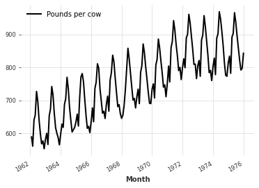
filler = MissingValuesFiller()
filled = filler.transform(incomplete_series, method="quadratic")

filled.plot()

../_images/examples_02-data-processing_14_0.png

由于 MissingValuesFiller 默认封装了 pd.interpolate，因此我们在调用 transform() 时也可以向 pd.interpolate() 函数提供参数

[8]:

filled = filler.transform(incomplete_series, method="quadratic")
filled.plot()

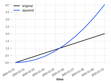
../_images/examples_02-data-processing_16_0.png

`Mapper` 和 `InvertibleMapper`：一种特殊的转换器¶

有时您可能想对数据执行一个简单的 map() 函数。这也可以使用数据转换器来完成。Mapper 接受一个函数并在调用 transform() 时将其逐元素应用于数据。

InvertibleMapper 还允许在创建时指定一个逆函数（如果存在），并提供 inverse_transform() 方法。

[9]:

lin_series = linear_timeseries(start_value=0, end_value=2, length=10)

squarer = Mapper(lambda x: x**2)
squared = squarer.transform(lin_series)

lin_series.plot(label="original")
squared.plot(label="squared")
plt.legend()

[9]:

<matplotlib.legend.Legend at 0x7ff5e3826c10>

../_images/examples_02-data-processing_18_1.png

更复杂（且有用）的变换¶

在之前使用的 Monthly Milk Production 数据集中，月份之间的一些差异来自于某些月份包含的天数多于其他月份，导致这些月份的牛奶产量更大。这使得时间序列更复杂，因此更难预测。

[10]:

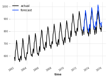
training, validation = series.split_before(pd.Timestamp("1973-01-01"))

model = ExponentialSmoothing()
model.fit(training)
forecast = model.predict(36)

plt.title(f"MAPE = {mape(forecast, validation):.2f}%")
series.plot(label="actual")
forecast.plot(label="forecast")
plt.legend()

[10]:

<matplotlib.legend.Legend at 0x7ff5e3bcc790>

../_images/examples_02-data-processing_20_1.png

为了考虑这一事实并获得更好的性能，我们可以选择

将时间序列转换为表示每个月的日均牛奶产量（而不是每月的总产量）
进行预测
反转变换

让我们看看如何使用 InvertibleMapper 和 pd.timestamp.days_in_month 实现这一点

（想法来源于 “预测：原理与实践”，作者：Hyndman 和 Athanasopoulos）

为了变换时间序列，我们必须将一个月度值（数据点）除以该值对应时间戳所在月份的天数。

map()（以及 Mapper / InvertibleMapper）通过允许应用一个变换函数使得这一点很方便，该函数使用值及其时间戳来计算新值：f(timestamp, value) = new_value

[11]:

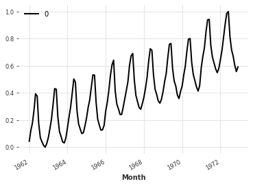
# Transform the time series
toDailyAverage = InvertibleMapper(
    fn=lambda timestamp, x: x / timestamp.days_in_month,
    inverse_fn=lambda timestamp, x: x * timestamp.days_in_month,
)

dailyAverage = toDailyAverage.transform(series)

dailyAverage.plot()

../_images/examples_02-data-processing_23_0.png

[12]:

# Make a forecast
dailyavg_train, dailyavg_val = dailyAverage.split_after(pd.Timestamp("1973-01-01"))

model = ExponentialSmoothing()
model.fit(dailyavg_train)
dailyavg_forecast = model.predict(36)

plt.title(f"MAPE = {mape(dailyavg_forecast, dailyavg_val):.2f}%")
dailyAverage.plot()
dailyavg_forecast.plot()
plt.legend()

[12]:

<matplotlib.legend.Legend at 0x7ff5e3dd1ac0>

../_images/examples_02-data-processing_24_1.png

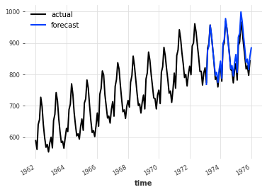
[13]:

# Inverse the transformation
# Here the forecast is stochastic; so we take the median value
forecast = toDailyAverage.inverse_transform(dailyavg_forecast)

[14]:

plt.title(f"MAPE = {mape(forecast, validation):.2f}%")
series.plot(label="actual")
forecast.plot(label="forecast")
plt.legend()

[14]:

<matplotlib.legend.Legend at 0x7ff5e3fbb280>

../_images/examples_02-data-processing_26_1.png

链式变换：引入 `Pipeline`¶

现在假设我们既想应用上述变换（日均化），又想将数据集重缩放到 0 到 1 之间以便使用基于神经网络的预测模型。与其分别应用这两个变换，然后再分别反转它们，我们可以使用一个 Pipeline。

[15]:

pipeline = Pipeline([toDailyAverage, scaler])
transformed = pipeline.fit_transform(training)
transformed.plot()

../_images/examples_02-data-processing_28_0.png

如果流水线中的所有变换都是可逆的，那么 Pipeline 对象也是可逆的。

[16]:

back = pipeline.inverse_transform(transformed)
back.plot()

../_images/examples_02-data-processing_30_0.png

现在回想一下来自 monthly-milk-incomplete.csv 的不完整序列。假设我们想将所有预处理步骤封装到一个 Pipeline 中，包括：一个用于填充缺失值的 MissingValuesFiller，以及一个用于将数据集缩放到 0 到 1 之间的 Scaler。

[17]:

incomplete_series = MonthlyMilkIncompleteDataset().load()

filler = MissingValuesFiller()
scaler = Scaler()

pipeline = Pipeline([filler, scaler])
transformed = pipeline.fit_transform(incomplete_series)

假设我们已经训练了一个神经网络并生成了一些预测。现在，我们想将数据缩放回去。不幸的是，由于 MissingValuesFiller 不是一个 InvertibleDataTransformer（谁会想在结果中插入缺失值呢？！），反向变换将引发一个异常：ValueError: Not all transformers in the pipeline can perform inverse_transform。

令人沮丧吧？幸运的是，您不必从头开始重新运行所有内容，将 MissingValuesFiller 从 Pipeline 中排除。相反，您只需将 inverse_transform 方法的 partial 参数设置为 True。在这种情况下，反向变换将跳过不可逆的转换器来执行。

[18]:

back = pipeline.inverse_transform(transformed, partial=True)

处理多个 TimeSeries¶

通常，我们需要处理多个时间序列。DARTS 支持将 TimeSeries 序列作为转换器和流水线的输入，这样您就不必单独处理每个样本。此外，它会负责存储在变换不同时间序列时（例如，使用缩放器）每个缩放器使用的参数。

[19]:

series = MonthlyMilkDataset().load()
incomplete_series = MonthlyMilkIncompleteDataset().load()

multiple_ts = [incomplete_series, series[:10]]

filler = MissingValuesFiller()
scaler = Scaler()

pipeline = Pipeline([filler, scaler])
transformed = pipeline.fit_transform(multiple_ts)

for ts in transformed:
    ts.plot()

../_images/examples_02-data-processing_36_0.png

[20]:

back = pipeline.inverse_transform(transformed, partial=True)
for ts in back:
    ts.plot()

../_images/examples_02-data-processing_37_0.png

监控和并行处理数据¶

有时，我们可能还需要处理巨大的数据集。在这种情况下，按顺序处理每个样本可能需要相当长的时间。Darts 可以帮助监控变换，并在可能的情况下并行处理多个样本。

在每个转换器或流水线中设置 verbose 参数时，将创建一些进度条

[21]:

series = MonthlyMilkIncompleteDataset().load()

huge_number_of_series = [series] * 10000

scaler = Scaler(verbose=True, name="Basic")

transformed = scaler.fit_transform(huge_number_of_series)

现在我们知道需要等待多久了。但是，由于没有人喜欢浪费时间等待，我们可以利用机器的多个核心并行处理数据。我们可以通过设置 n_jobs 参数来实现（用法与 sklearn 中相同）。

注意：加速效果与可用核心数量和变换的“CPU密集度”密切相关。

[22]:

# setting n_jobs to -1 will make the library using all the cores available in the machine
scaler = Scaler(verbose=True, n_jobs=-1, name="Faster")
scaler.fit(huge_number_of_series)
back = scaler.transform(huge_number_of_series)

[ ]:

多个时间序列、预训练模型和协变量

静态协变量

使用 DataTransformer 和 Pipeline 进行数据（预）处理¶

DataTransformer 抽象¶