层级协调 - 以澳大利亚旅游数据集为例
在本 notebook 中,我们将演示层级协调。我们将使用澳大利亚旅游数据集(原始数据来自这里),该数据集包含按地区、出行目的和城市/非城市类型划分的月度旅游人数。
我们将使用 Rob Hyndman 的书这里中介绍的技术,我们将看到,使用 Darts,仅需几行代码即可完成预测的协调。
首先,进行一些导入
[1]:
# fix python path if working locally
from utils import fix_pythonpath_if_working_locally

fix_pythonpath_if_working_locally()
%matplotlib inline
[2]:
from itertools import product

import matplotlib.pyplot as plt

from darts import concatenate
from darts.dataprocessing.transformers import MinTReconciliator
from darts.datasets import AustralianTourismDataset
from darts.metrics import mae
from darts.models import LinearRegressionModel, Theta
/Users/dennisbader/miniconda3/envs/darts310_test/lib/python3.10/site-packages/statsforecast/utils.py:237: FutureWarning: 'M' is deprecated and will be removed in a future version, please use 'ME' instead.
  "ds": pd.date_range(start="1949-01-01", periods=len(AirPassengers), freq="M"),
加载数据
下面,我们加载一个 TimeSeries,它是多元的(即包含多个组件)。为了简单起见,我们直接使用 Darts 数据集 AustralianTourismDataset,但我们也可以使用 TimeSeries.from_dataframe(df),提供一个 DataFrame df,其中每列代表一个组件,每行代表一个时间戳。
[3]:
tourism_series = AustralianTourismDataset().load()
该序列包含几个组件
一个名为
"Total"的组件,每个地区一个组件(
"NSW"、"VIC"等)每个旅游原因一个组件(
"Hol"代表度假,"Bus"代表商务等)每个(地区、原因)对一个组件(名称如
"NSW - hol"、"NSW - bus"等)每个(地区、原因、<城市>)元组一个组件,其中 <城市> 可以是
"city"或"noncity"。因此,这些组件的名称如"NSW - hol - city"、"NSW - hol - noncity"、"NSW - bus - city"等。
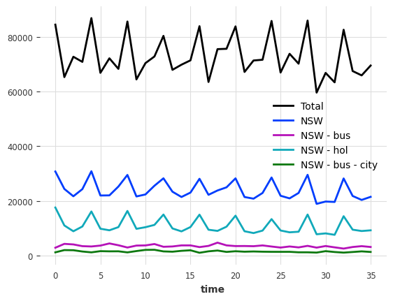
让我们绘制其中几个
[4]:
tourism_series[["Total", "NSW", "NSW - bus", "NSW - hol", "NSW - bus - city"]].plot()
[4]:
<Axes: xlabel='time'>
检查层级结构
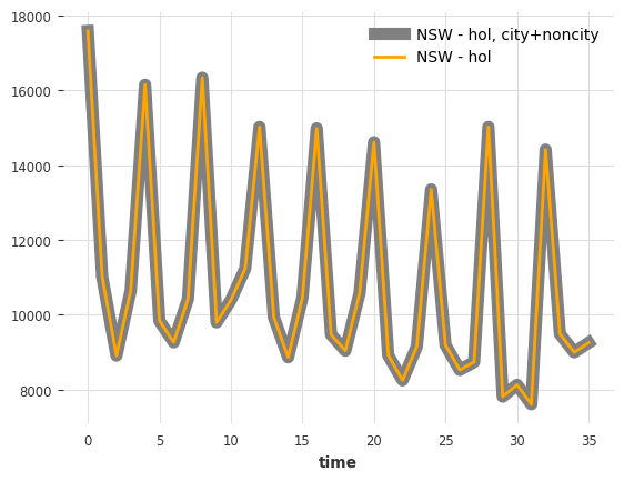
这些组件中有一些以特定方式相加。例如,新南威尔士州的度假旅游总数可以分解为新南威尔士州“城市”和“非城市”度假旅游的总和
[5]:
sum_city_noncity = (
    tourism_series["NSW - hol - city"] + tourism_series["NSW - hol - noncity"]
)
sum_city_noncity.plot(label="NSW - hol, city+noncity", lw=8, color="grey")
tourism_series["NSW - hol"].plot(color="orange")
[5]:
<Axes: xlabel='time'>
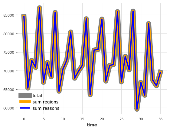
同样,按地区和原因的总和都加起来等于总计
[6]:
reasons = ["Hol", "VFR", "Bus", "Oth"]
regions = ["NSW", "VIC", "QLD", "SA", "WA", "TAS", "NT"]
city_labels = ["city", "noncity"]

tourism_series["Total"].plot(label="total", lw=12, color="grey")
tourism_series[regions].sum(axis=1).plot(label="sum regions", lw=7, color="orange")
tourism_series[reasons].sum(axis=1).plot(label="sum reasons", lw=3, color="blue")
[6]:
<Axes: xlabel='time'>
所以总的来说,我们的层级结构如下所示

编码层级结构
现在我们将以 Darts 能够理解的方式编码层级结构本身。这很简单:层级结构只需表示为一个 dict,其中键是组件名称,值是包含该组件在该层级结构中父组件的列表。
例如,参照上图
"Hol"映射到["Total"],因为它在左侧树中是"Total"的子节点。"NSW - hol"映射到["Hol", "NSW"],因为它既是"Hol"(在左侧树中)的子节点,也是"NSW"(在右侧树中)的子节点。"NSW - bus - city"映射到["NSW - bus"],因为它在右侧树中是"NSW - bus"的子节点。等等…
因此,除 "Total" 外,所有组件都将作为层级字典中的一个键出现。由于组件数量较多(96个),我们将不手动构建此字典,而是以编程方式构建
[7]:
hierarchy = dict()

# Fill in grouping by reason
for reason in reasons:
    hierarchy[reason] = ["Total"]

# Fill in grouping by region
for region in regions:
    hierarchy[region] = ["Total"]

# Fill in grouping by (region, reason)
for region, reason in product(regions, reasons):
    hierarchy[f"{region} - {reason.lower()}"] = [reason, region]

# Fill in grouping by (region, reason, <city>)
for region, reason, city in product(regions, reasons, city_labels):
    hierarchy[f"{region} - {reason.lower()} - {city}"] = [
        f"{region} - {reason.lower()}"
    ]
作为健全性检查,让我们看看层级中几个组件的映射
[8]:
for component in ["Hol", "NSW - hol", "NSW - bus - city"]:
    print(f"{component} -> {hierarchy[component]}")
Hol -> ['Total']
NSW - hol -> ['Hol', 'NSW']
NSW - bus - city -> ['NSW - bus']
很好,这看起来符合预期。
在 Darts 中,层级是 TimeSeries 对象的属性。现在我们可以将我们的层级结构嵌入到我们的 TimeSeries 中。我们使用 with_hierarchy() 方法来实现,但我们也可以在序列构建时指定层级结构;例如,在 TimeSeries.from_dataframe() 工厂方法中提供一个 hierarchy 参数。
[9]:
tourism_series = tourism_series.with_hierarchy(hierarchy)
使用多元模型进行预测
现在我们有一个多元时间序列,其中包含层级信息。让我们将其分割为训练/评估部分。我们将保留最后12个月作为验证集。
[10]:
train, val = tourism_series[:-12], tourism_series[-12:]
现在获取预测结果就像使用 Darts 支持多元序列的模型一样简单
[11]:
model = LinearRegressionModel(lags=12)
model.fit(train)
pred = model.predict(n=len(val))
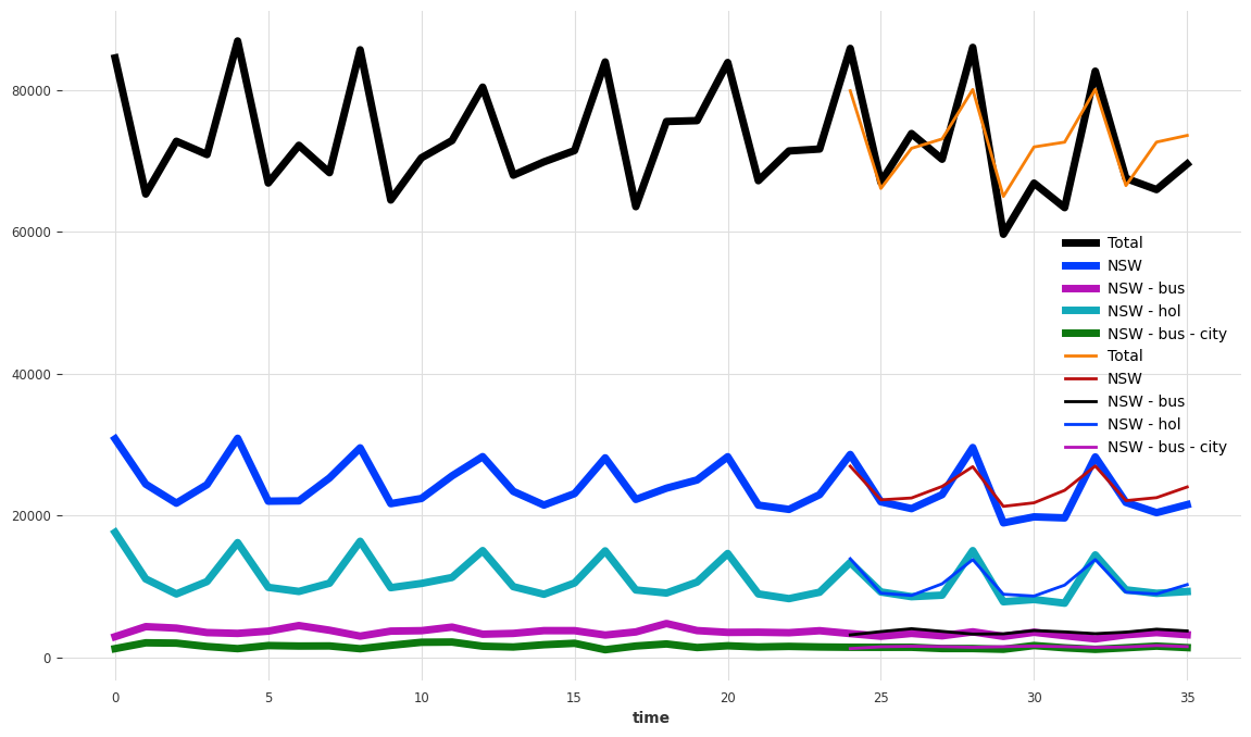
让我们看看我们的预测结果
[12]:
components_to_show = ["Total", "NSW", "NSW - bus", "NSW - hol", "NSW - bus - city"]
plt.figure(figsize=(14, 8))
tourism_series[components_to_show].plot(lw=5)
pred[components_to_show].plot(lw=2)
[12]:
<Axes: xlabel='time'>
我们也计算不同层级的准确性(MAE,对多个组件取平均)
[13]:
# we pre-generate some of the components' names
regions_reasons_comps = list(
    map(lambda t: f"{t[0]} - {t[1].lower()}", product(regions, reasons))
)

regions_reasons_city_comps = list(
    map(
        lambda t: f"{t[0]} - {t[1].lower()} - {t[2]}",
        product(regions, reasons, city_labels),
    )
)


def measure_mae(pred):
    def print_mae_on_subset(subset, name):
        print(f"mean MAE on {name}: {mae(pred[subset], val[subset]):.2f}")

    print_mae_on_subset(["Total"], "total")
    print_mae_on_subset(reasons, "reasons")
    print_mae_on_subset(regions, "regions")
    print_mae_on_subset(regions_reasons_comps, "(region, reason)")
    print_mae_on_subset(regions_reasons_city_comps, "(region, reason, city)")


measure_mae(pred)
mean MAE on total: 4311.00
mean MAE on reasons: 1299.87
mean MAE on regions: 815.08
mean MAE on (region, reason): 315.89
mean MAE on (region, reason, city): 191.85
协调预测
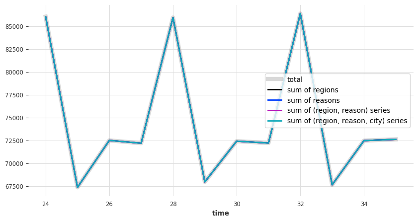
首先,让我们看看我们当前的“原始”预测结果是否相加一致
[14]:
def plot_forecast_sums(pred_series):
    plt.figure(figsize=(10, 5))

    pred_series["Total"].plot(label="total", lw=6, alpha=0.3, color="grey")
    pred_series[regions].sum(axis=1).plot(label="sum of regions")
    pred_series[reasons].sum(axis=1).plot(label="sum of reasons")
    pred_series[regions_reasons_comps].sum(axis=1).plot(
        label="sum of (region, reason) series"
    )
    pred_series[regions_reasons_city_comps].sum(axis=1).plot(
        label="sum of (region, reason, city) series"
    )

    legend = plt.legend(loc="best", frameon=1)
    frame = legend.get_frame()
    frame.set_facecolor("white")


plot_forecast_sums(pred)
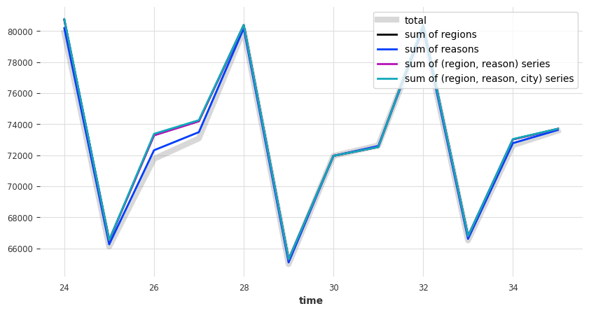
看来它们并不相加一致。因此,让我们协调它们。我们将使用 darts.dataprocessing.transformers 中可用的一些转换器来完成此操作。这些转换器可以执行*后验*协调(即,在获得预测结果后进行协调)。我们有以下方法可供选择
BottomUpReconciliator执行自下而上的协调,只需将层级结构中的每个组件重设为其子组件的总和(API 文档)。TopDownReconciliator执行自上而下的协调,它使用历史比例将聚合预测结果分解到层级结构的下方。这个转换器需要使用历史值(即训练序列)调用fit()来学习这些比例(API 文档)。MinTReconciliator是一种执行“最优”协调的技术,详情见这里。这个转换器有几种不同的工作方式,列在API 文档中。
下面,我们使用 MinTReconciliator 的 wls_val 变体
[15]:
reconciliator = MinTReconciliator(method="wls_val")
reconciliator.fit(train)
reconcilied_preds = reconciliator.transform(pred)
现在让我们检查协调后的预测结果是否如我们预期的那样相加一致
[16]:
plot_forecast_sums(reconcilied_preds)
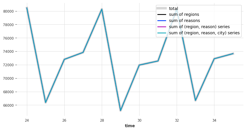
看起来不错 - 那么 MAE 误差呢
[17]:
measure_mae(reconcilied_preds)
mean MAE on total: 4205.92
mean MAE on reasons: 1294.87
mean MAE on regions: 810.68
mean MAE on (region, reason): 315.11
mean MAE on (region, reason, city): 191.36
与之前相比,MAE 略有增加(例如在总计层级),而在其他更细粒度的层级则略有下降。这是协调的典型情况:它可能会增加误差,但在某些情况下也可能减少误差。
替代方法:独立预测组件
上面,我们只是在我们的多元序列上拟合了一个单一的多元模型。这意味着每个维度的预测都使用了所有其他维度的(滞后)值。下面,为了示例起见,我们重复实验,但使用“局部”模型独立预测每个组件。我们使用一个简单的 Theta 模型,并将所有预测结果连接到一个单一的多元 TimeSeries 中
[18]:
preds = []
for component in tourism_series.components:
    model = Theta()
    model.fit(train[component])
    preds.append(model.predict(n=len(val)))

pred = concatenate(preds, axis="component")
/Users/dennisbader/miniconda3/envs/darts310_test/lib/python3.10/site-packages/statsmodels/tsa/holtwinters/model.py:917: ConvergenceWarning: Optimization failed to converge. Check mle_retvals.
  warnings.warn(
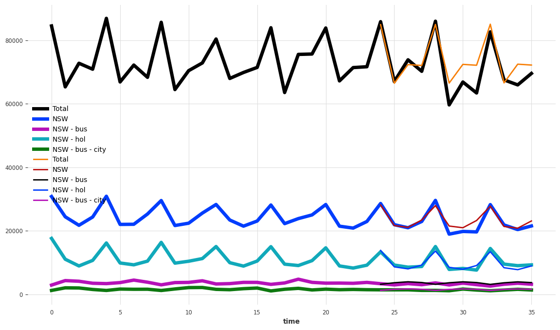
让我们绘制几个预测结果,并显示 MAE 误差
[19]:
plt.figure(figsize=(14, 8))
tourism_series[components_to_show].plot(lw=5)
pred[components_to_show].plot(lw=2)
measure_mae(pred)
mean MAE on total: 3294.38
mean MAE on reasons: 1204.76
mean MAE on regions: 819.13
mean MAE on (region, reason): 329.39
mean MAE on (region, reason, city): 195.16
正如预期的那样,这些预测结果也不相加一致
[20]:
plot_forecast_sums(pred)
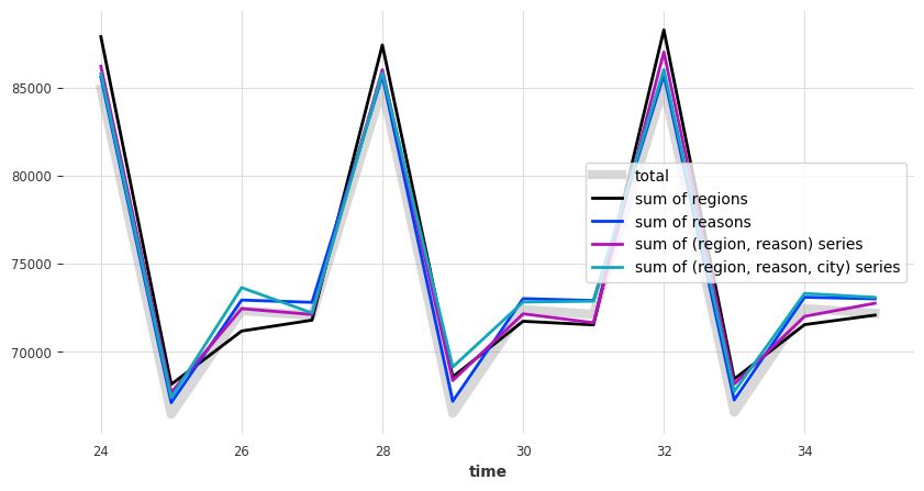
让我们使用 MinTReconciliator 使它们相加一致
[21]:
reconciliator = MinTReconciliator(method="wls_val")
reconciliator.fit(train)
reconcilied_preds = reconciliator.transform(pred)

plot_forecast_sums(reconcilied_preds)
measure_mae(reconcilied_preds)
mean MAE on total: 3349.33
mean MAE on reasons: 1215.91
mean MAE on regions: 782.26
mean MAE on (region, reason): 316.39
mean MAE on (region, reason, city): 199.92